A deep learning approach for person identification using ear biometrics

Abstract

Automatic person identification from ear images is an active field of research within the biometric community. Similar to other biometrics such as face, iris and fingerprints, ear also has a large amount of specific and unique features that allow for person identification. In this current worldwide outbreak of COVID-19 situation, most of the face identification systems fail due to the mask wearing scenario. The human ear is a perfect source of data for passive person identification as it does not involve the cooperativeness of the human whom we are trying to recognize and the structure of ear does not change drastically over time. Acquisition of a human ear is also easy as the ear is visible even in the mask wearing scenarios. Ear biometric system can complement the other biometric systems in automatic human recognition system and provides identity cues when the other system information is unreliable or even unavailable. In this work, we propose a six layer deep convolutional neural network architecture for ear recognition. The potential efficiency of the deep network is tested on IITD-II ear dataset and AMI ear dataset. The deep network model achieves a recognition rate of 97.36% and 96.99% for the IITD-II dataset and AMI dataset respectively. The robustness of the proposed system is validated in uncontrolled environment using AMI Ear dataset. This system can be useful in identifying persons in a massive crowd when combined with a proper surveillance system.

Introduction

The demand for secured automated identity system has intensified the research in the fields of computer vision and intelligent systems. Most of the human identification systems make use of the biometrics because of their invariance over time, easiness to acquire, and uniqueness for each individual. The physical or behavioral traits including face, iris, fingerprint, palmprint, hand geometry, voice, and signature are the most commonly used biometrics for human identification. Many research works for the biometric systems have been implemented successfully and are now available for public use. These biometric systems are mostly used for human authentication purposes. For human identification, most of this biometrics requires the cooperation from the corresponding human in order to acquire the biometric traits.

Due to the current COVID-19 pandemic situation around the world, the entire human community is becoming a mask wearing community. Because of this reason, the face recognition systems suffer a lot and there is need for rework in the existing systems. Fingerprint and palmprint based recognition are not suitable in this COVID-19 scenario because of its contact based feature extraction. Iris based recognition systems are costly because of the special sensors needed for extracting the features in Iris. Also, all the above discussed biometric systems require the co-operation of the person to get identified. These biometric systems are less likely to be feasible for person identification in massive crowd environments such as railway stations, museums, shopping malls etc. … So, a contactless, non co-operative biometric system such as ear biometrics is the need of this hour.

The human ear preserves stable structure since birth, and it is unique for every individual. Also, the acquisition method for the human ear is contactless and nonintrusive and also it does not involve the cooperativeness of the human whom we are trying to recognize. Ear biometric can serve as a supplement for other biometric modalities in automatic recognition systems and provide identity cues when other information is unreliable or even unavailable. In surveillance applications, when face recognition may struggle with profile faces, the ear can serve as a source of information on the identity of human in the surveillance footage [1–5]. So, the automated human identification using ear images has been increasingly studied for its possible commercial applications.

Many medical studies have shown that significant changes in the shape of the ear happen before the age of 8 years and after the age of 70 years. The color distribution of ear is almost uniform. The position of the ear is almost in the middle of the profile face. Ear data can be captured even without the awareness of the subject from a distance. A simple digital camera such as CCTV camera is suitable for capturing the ear images. Fig. 1 shows the sample arrangement of the ear biometric system. The CCTV-1 captures a clear shot of profile face without much tilt or rotation of the ear. CCTV-2 and CCTV-3 are used for capturing more profile photos for multiple images of the same person to form the feature matrices.

Fig. 1.

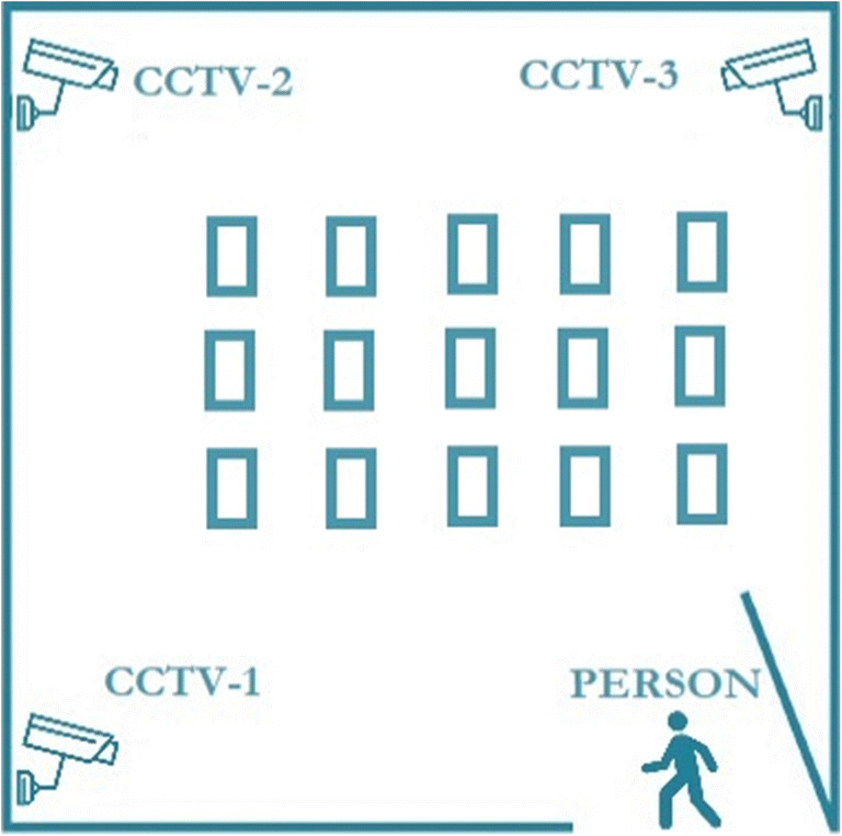
Sample Environment of Ear Biometric System

Human ear contains stable and reliable information as well as shape structure that does not show drastic changes with age. Fig. 2 shows the visible structure of the human ear and its various morphological components including: helix, antihelix, tagus, antitragus, lobe, concha and other parts. While the visible outer structure is comparatively simple, the changes between two ears is evident enough even for identical twins [6]. Also, the human ear image has uniform color distribution for the ear surface and the ear images are invariant to facial expressions. Therefore, the analysis of ear images for extracting such unique and distinguishable features to identify individuals and verify their identities is an active research topic and an emerging intelligent biometric application [7]. Longitudinal studies from India [8] and Europe [9–11] have revealed that the length of the ear increases with age for human, while the width and structure remains relatively constant.

Fig. 2.

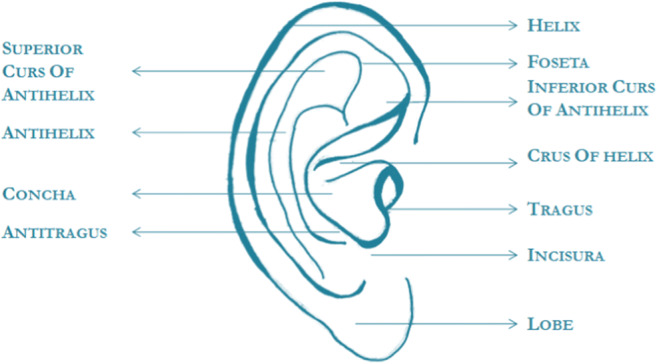
Visible structure of Human Ear

The research works on automatic human ear recognition have started during the mid 1990s. In the year 1996, for ear description, Burge and Burger have used adjacency graphs computed from Voronoi diagrams of the ears curve segments [12]. Moreno et al. developed the first fully automated ear recognition procedure using geometric characteristics of the ear and a compression network [13]. Most of the research works in the ear recognition falls in any one of the following approaches such as (a) Geometric approaches (b) Holistic Approaches (c) Local Approaches (d) Hybrid approaches. Geometric techniques extract the geometrical characteristics of the ear, such as shape, position of specific ear parts and their relationships. Holistic approaches consider the ear as a whole and describe the global properties of the ear. Local approaches portray the local parts or the local appearance of the ear. Hybrid approaches combine elements from all categories or rely on multiple representations to improve the performance.

Many geometric approaches for human ear recognition uses the coordinates of characteristic ear points, morphology descriptors of the ear shape and the structure of wrinkles [13], relationships between the selected points on the contour of the ear [14], angle-based contour representations [15], geometric properties of subparts of ears [16] . Detecting the proper edge of the ear in the presence of illumination variations and noise and locating the specific ear point in an occluded ear deteriorate the performance of the geometric approaches [17].

Force field transform is one of the most popular holistic approaches for human ear recognition. This transform computes a force field from the ear image by treating the pixels as sources of a Gaussian force field. The properties of force field are used to compute similarities between ear images [18–20]. The other holistic approaches are based on the linear and nonlinear subspace projection techniques which include Principal Component Analysis (PCA) [21], Independent Component Analysis (ICA) [22], Non-Negative Matrix Factorization (NMF) [23], Linear Discriminant Analysis (LDA) [24], Null Kernel Discriminant Analysis (NKDA) [25] etc. Normalization techniques are mandatory prior to feature extraction in holistic approaches to correct the changes in ear appearance because of the changes in pose and illumination.

Local approaches mainly extract the texture information around the detected key points or over the entire image. The local approaches include scale invariant feature transform (SIFT), speeded up robust features (SURF), histograms of oriented gradients (HOG), local binary patterns (LBP), Gabor or log-Gabor filters and other types of wavelet representations [26–32]. For the experimentation of different local features, most of the researchers have used the IITD-II Ear Dataset.

Hybrid approaches use multiple representations to increase the recognition performance. Kumar and Chan adopted the sparse representation classification algorithm and applied it to local gray-level orientation features [33]. Recently, deep learning methods are mostly used in the field of pattern recognition because of their ability to perform automatic feature extraction from raw data. The first deep network, LeNet is designed for handwritten and machine-printed character recognition [34]. Currently, deep learning finds its usage in different fields such as, plant disease classification [35], medical applications [36, 37], speech processing [38], etc. Dodge et al. used many deep networks such as AlexNet, VGGNet etc. for unconstrained ear recognition [39]. They have worked on AWE and CVLE ear datasets. Galdámez et al. used a Convolutional Neural Network for recognizing the ears from Avila’s Police School Dataset and Bisite Videos Dataset [40].

In this proposed work, we are concentrating on recognizing humans based on their ear profiles using deep learning methods. We have used the IITD-II dataset to analyze the performance of the designed deep neural network. According to our knowledge, so far, no research has been published, which explores the capability of deep convolutional neural networks on IITD-II dataset. The influence of the network parameters such as learning rate, kernel size and the activation functions on ear recognition is also studied in detail. The potential efficiency of the newly designed deep neural network is verified on AMI dataset.

Materials and methods

Convolutional neural networks (CNNs) are deep artificial neural networks that are used primarily to classify images, to recognize visual patterns directly from pixel images with minimal preprocessing. CNNs observe the images as volumes; i.e. three-dimensional objects including width and height and depth. The CNNs comprise of convolutional Layers, Sub sampling Layers and fully connected Layers. The CNN architecture used in the proposed work is shown in Fig. 3.

Fig. 3.

Architecture of the proposed deep CNN for IITD-II dataset

It consists of six levels of convolutional layers. After every convolutional layer, a sub sampling layer is introduced to reduce the dimension of the feature maps. After every two convolutional layers, a batch normalization layer is introduced to improve the stability of the network. The output layer is a fully connected layer contains 221 neurons which describe the class labels. The designed deep CNN for IITD-II dataset has 677,325 learnable parameters.

Components of CNN architecture

The primary purpose of the convolutional layer is to extract features from the input image by employing the convolution operation with the kernel. Convolution protects the spatial relationship between pixels. The convolutional kernel slides over the input image and performs the convolution operation to produce a feature map. The convolution of another kernel over the same image will result in a different feature map. The addition of more convolutional layers, results in learning the abstract features which are not visible. The size of the feature map obtained at the output of the convolutional layer is depicted in Eq. 1

$$y=\left(\frac{x-w+2p}{s}\right)+1$$ 1

where x, y represents the dimensions of the input and output of the convolutional layer respectively, w be the kernel size, p be the padding value and s be the stride value. In this work, padding and stride value is set to 1 for the entire experimentation.

The activation function is a vital function in a CNN making it capable of learning and performing more complex tasks. Activation function performs nonlinear transformation by deciding whether the information received by the neuron is relevant or not. If the information is irrelevant, it should be ignored. The commonly used activation functions are sigmoid, tanh, rectified linear unit (ReLU), softmax etc. The ReLU is the most used activation function in almost all the convolutional neural networks. ReLU activation is half rectified (from bottom). The activation function f(y) is zero when y is less than zero and f(y) is equal to y when y is greater than or equal to zero. ReLU is not bounded and it ranges between (0 to ∞). On the other hand, ELU and SELU have a small slope for negative values. Instead of a straight line, ELU uses a log curve and SELU uses a scaled log curve. The sigmoid activation function is traditionally used in neural networks and is bounded between (0 to 1). Therefore, it is especially used for models where we have to predict the probability as an output. The tanh activation function on the other hand is the bipolar version of the sigmoid activation function and is bounded between (−1 to +1). The advantage of tanh is that the negative inputs will be mapped strongly negative and the zero inputs will be mapped near zero. The softmax function is a more generalized version of the sigmoid activation function which is used for multiclass classification. The mathematical expressions for the RELU, ELU, SELU, sigmoid, tanh and softmax activations are tabulated in Table 1 and also, the activation functions are depicted in Fig. 4.

Table 1.

Mathematical Expressions of various activation functions

Activation Functions	Mathematical Expressions
ReLU	f(y) = max (0, y)
ELU	$f\left(y\right)=\left\{\begin{array}{cc}y& y>0\\ \alpha \left(e^y-1\right)& y\le 0\end{array}\right)$ where α > 0
SELU	$f\left(y\right)=\lambda \left\{\begin{array}{cc}y& y\ge 0\\ \alpha \left(e^y-1\right)& y<0\end{array}\right)$ where λ > 1 and α > 0
Sigmoid	$f\left(y\right)=\frac{1}{1+e^{-y}}$
Tanh	$f\left(y\right)=\frac{2}{1+e^{-2y}}-1$
Softmax	$f\left(y_j\right)=\frac{e^{y_j}}{\sum _{i=1}^m{e}^{y_i}}$ where m represents number of classes

Fig. 4.

Activation Functions (a) RELU (b) ELU (c) SELU (d) Sigmoid (e) Tanh

The next layer in a convolutional network is the subsampling layer. A subsampling layer mostly follows a convolution layer in CNN. The role of the subsampling layer is to downsample the output of a convolution layer in both height and width. The primary function of a subsampling later is to reduce the learnable parameters of the network. This also reduces overfitting and thereby increases the overall performance and accuracy of the network. We have used the Max Subsampling in our experimentation.

A batch normalization layer normalizes each input channel across a mini-batch. It is used to speed up the training of CNNs and to reduce the sensitivity of network initialization. The layer first normalizes the activations of each channel by subtracting the mini-batch mean and dividing by the mini-batch standard deviation.

The fully connected layer in a CNN connects every neuron in the previous layer to every neuron on the current layer. The activations can be computed with a matrix multiplication followed by a bias offset. After multiple layers of convolution and padding, we require the output in the form of a class. The convolution and subsampling layers extract features and reduce the number of parameters from the original image. The number or neurons in the last fully connected layer is same as the number of classes to be predicted. The output layer has a loss function like categorical cross-entropy, to compute the error in prediction as shown in Eq. (2)

$$J\left(\phi \right)=-\frac{1}{M}\sum _{\forall X}\sum _j{y}_j\mathit{log}{o}_j^k+\left(1-y_j\right)log\left(1-o_j^k\right)$$ 2

where M represents the number of classes, y_j and o_j represents the actual and predicted labels respectively. k represents the corresponding layer. After the prediction, the back propagation algorithm updates the weight and biases for error and loss reduction.

Dropout is also a regularization technique used in neural networks. Deep neural networks are prone to overfitting. Dropout technique drops a set of randomly selected nodes during every iteration of gradient descent. Gradient descent minimizes an objective function J(φ) with respect to the model’s parameter φ by updating the parameters in the opposite direction of the gradient. The learning rate η determines the size of the steps for reaching a (local) minimum. Gradient descent is broadly categorized into three types such as Batch gradient descent, stochastic gradient descent and mini-batch gradient descent based on how much data is used to compute the gradient of the objective function. In our work, we have used the batch gradient descent algorithm for learning and RmsProp optimizer for updating the weights. Optimizers update the weight parameters to minimize the loss function. RMSProp optimizer (http://www.cs.toronto.edu/~tijmen/csc321/slides/lecture_slides_lec6.pdf) tries to resolve the radically diminishing learning rates by using a moving average of the squared gradient. It utilizes the magnitude of the recent gradient descents to normalize the gradient. The weight update rule is given in Eq. 3.

$${\phi }_{i+1}={\phi }_i-\frac{\eta }{\sqrt{\left(1-\mathit{\gamma }\right){\nabla }_{{\phi }_i}^{2}J\left({\phi }_i\right)+\gamma {\nabla }_{{\phi }_i}J\left({\phi }_i\right)+ϵ}}{\nabla }_{{\phi }_i}J\left({\phi }_i\right)$$ 3

where γ is the decay term that takes value from 0 to 1. ${\nabla }_{{\phi }_i}$is the moving average of squared gradients.

Dataset used

IITD ear dataset

The IIT Delhi ear image database comprises of two sets of datasets namely IITD-I and IITD-II containing 125 different subjects and 221 different subjects respectively (https://www4.comp.polyu.edu.hk/~csajaykr/IITD/Database_Ear.htm). All the subjects in the database are in the age group 14–58 years. In our experimentation we have used the IITD-II dataset which contains 793 ear images with a resolution of 50 × 180 pixels. The sample images of this database are shown in Fig. 5.

Fig. 5.

Sample images of IITD-II Dataset

AMI dataset

AMI ear dataset consists of 700 ear images acquired from 100 different subjects in the age of 19–65 years (http://ctim.ulpgc.es/research_works/ami_ear_database/). Each subject has 7 images out of which 6 images are for the right ear and one image is for the left ear. Five images of the right ear for the subject looking forward, left, right, up and down, respectively and the sixth image of the right ear is for the subject is with a different camera focal length (Zoomed). The last image is for the left ear with the subject facing forward. All images have the resolution of 492 × 702 pixels. The sample images of AMI database is shown in Fig.6.

Fig. 6.

Sample images of AMI Dataset

Experiment results and discussions

In this work, we present a human ear recognition method based on deep CNN architecture. The simple deep learning architecture is designed keeping in mind the memory requirement for the end applications. The architecture given in Fig. 3 is used for the experimentation purpose. The details about the parameters of the proposed deep architecture are given in Table. 2.

Table 2.

Parameters for the designed deep network

Layer	Output Feature Map Size	Kernel Size	No. of Learnable Parameters
Conv Layer 1	180 × 50 × 8	3 × 3	224
Max Pool Layer 1	90 × 25 × 8	2 × 2	0
Conv Layer 2	90 × 25 × 16	3 × 3	1168
Batch Norm Layer 1	90 × 25 × 16	–	64
Max Pool Layer 2	45 × 12 × 16	2 × 2	0
Conv Layer 3	45 × 12 × 32	3 × 3	4640
Max Pool Layer 3	22 × 6 × 32	2 × 2	0
Conv Layer 4	22 × 6 × 64	3 × 3	18,496
Batch Norm Layer 2	22 × 6 × 64	–	256
Max Pool Layer 4	11 × 3 × 64	2 × 2	0
Conv Layer 5	11 × 3 × 128	3 × 3	73,856
Max Pool Layer 5	5 × 1 × 128	2 × 2	0
Conv Layer 6	5 × 1 × 256	3 × 3	295,168
Batch Norm Layer 3	5 × 1 × 256	–	1024
Flattening Layer	1280	–	0
Output Layer	221	–	283,101
Total No. of Learnable Parameters			677,997

For the entire experimentation in IITD-II dataset, 490 images are used for training purpose and 303 images are used for testing purpose. The entire experimentation is carried out for 10 times with different train and test samples and the average accuracy is presented in the paper. First, to fix a proper learning rate η, the experimentation is carried out with the kernel size 3 × 3 for all the convolutional layers for different epochs. The experimentation results are tabulated in Table 3.

Table 3.

Recognition Rate of IITD-II Dataset for different learning rates

No. of epochs	Recognition Rate (%)
	η = 0.001	η = 0.0001
100	92.73	90.43
200	92.07	91.42
500	93.07	92.07
1000	94.05	93.07

From Table 3, it is inferred that, the learning rate η= 0.001 provides a better result while using the RMSprop optimizer as indicated by Geoff Hinton (Lecture Notes).

For further experimentation, the learning rate is fixed as η= 0.001. To fix a better kernel size for the deep CNN, the experimentation is carried out using different kernel sizes. The kernel size 5 × 3 was chosen as part of experiment, to preserve the aspect ratio of the image. The experimentation results for different kernel sizes are tabulated in Table 4.

Table 4.

Recognition Rate of IITD-II Dataset for different kernel sizes

No. of epochs	Recognition Rate(%)
	Kernel Size
	3 × 3	5 × 5	5 × 3
100	92.73	92.41	91.75
200	92.07	90.42	91.09
500	93.07	85.48	89.77
1000	94.05	84.82	89.11

From Table 4, it is clear that the kernel size 3 × 3 performs better for the IITD-II dataset. Further experimentation is carried out by fixing the kernel size as 3 × 3.To improve the recognition rate further and to avoid the overfitting, it is decided to augment the input images by tilting them to a certain angle. Table 5 shows the recognition rate by varying the degree of rotation.

Table 5.

Recognition Rate of IITD-II Dataset for different degree of rotation

No. of epochs	Recognition Rate(%)
	Kernel Size
	2°	5°	7°	10°
1000	93.07	94.72	95.38	94.38

Table 5 clearly indicates that, augmentation with the rotation angle 7^°, performs better than the other degrees of rotation. Upto this, the experimentation is carried out using the ReLU activation function. A sample training performance curve for the deep learning model with augmentation of 7^° rotation and ReLU activation function is shown in Fig. 7.

Fig. 7.

Sample Training Performance of designed deep network

To find out which activation function suits ear recognition, we experimented with different activation functions such as ReLU, Exponential Linear Unit (ELU), Scaled Exponential Linear Unit (SELU), sigmoid and tanh activation functions on IITD-II dataset. The performance of various activation functions on IITD-II dataset is depicted in Fig. 8.

Fig. 8.

Performance of various activation functions

From Fig. 8, it is evident that, the activation function tanh outperforms others in ear recognition. Since our model consists of lesser number of layers, the usage of bounded activation function tanh on the model does not suffer from vanishing gradient problem. Also from the experimentation, we observed that, sigmoid activation function suffers from overfitting. For the tanh activation function, we achieved a recognition rate of 97.36% for the IITD-II dataset which is comparable with other state of art methods as shown in Table 6. In the mentioned state-of-art methods, the train test ratio maintained is 67:33 which is same as our method.

Table 6.

Performance Comparison of IITD-II dataset with state of art methods

Method	Recognition Rate (%)
Log-Gabor Feature with Weighted Sum matching [30]	95.93
Monogenic Log-Gabor [41]	96.34
SUMrule based fusion [32]	92.40
Nonlinear curvelet features and k-NN [31]	96.22
BSIF descriptor [42]	97.30
Proposed Deep CNN	97.36

The feature maps for the first two convolutional layers are shown in Fig. 9. The ability of the proposed deep CNN architecture is further tested with AMI Ear dataset. Out of the 700 ear images 600 images were trained and 100 images were tested. The input image is resized to 176 × 123 to fit into the Deep CNN architecture to maintain the aspect ratio. The recognition rate achieved is 96.99% for 1000 epochs with tanh activation function and is compared with the existing methods shown in Table 7.

Fig. 9.

Feature maps (a) convolution layer 1 (b) convolution layer 2

Table 7.

Performance Comparison of AMI dataset with state of art methods

Method	Recognition Rate (%)
Local Binary Patterns [29]	73.71
MAML + CNN [43]	93.96
DCGAN+VGG16 [44]	96.00
Proposed Deep CNN	96.99

From Tables 6 and 7 it is inferred that the proposed deep CNN architecture provides comparable performance with the state-of-art methods. Since the number of learnable parameters is limited to 677,997, the memory requirement for this model is approximately 5.17 MB.

To analyze the performance of the trained model in uncontrolled environment, we carried out the experimentation further by applying different transformations such as rotation, illumination and noise addition on the test images. Since, IITD-II dataset contains cropped ear images; we have chosen the AMI Ear dataset for carrying out the experimentation in uncontrolled environment. Also, the ear images in AMI Ear Dataset resemble the real environment images. The sample images of the different transformations applied on the test images of AMI Ear dataset are shown in Fig. 10.

Fig. 10.

Sample images of the different transformations applied on test images of AMI Ear dataset. (a) Original Image (b) Rotated at various angles (c) Under different illumination conditions (d) Gaussian noise added with different variance

We have conducted exhaustive experimentations on the test images by rotating them in various angles, under different illumination conditions and by adding random noise individually. As Gaussian noise arises in digital images during acquisition, here the experiment is conducted by adding Gaussian noise with different variances. The performance of the trained model on the uncontrolled environment is given in Table 8.

Table 8.

Performance of the trained model on uncontrolled environment in AMI dataset

Recognition Rate (%)
Rotation				Illumination				Noise				R + I + N*
5°	7°	9°	11°	50%	70%	110%	130%	σ = 1	σ = 3	σ = 5	σ = 7
94.99	96.99	92.99	91.99	94.99	96.99	91.99	85.99	96.99	95.99	95.99	89.99	91.99

^* R + I + N indicated testing done in combined manner

From Table 8, it is clear that, this deep CNN model is capable of recognizing human from the ear images even under different transformations. To test the robustness of the system, the test is carried out by performing all the transformations on the test images in a combined manner with a rotation of 9^°,70% illumination and random noise added with σ = 3. Even under this scenario, the trained model gives an acceptable performance of 91.99% accuracy. From these experimentations we claim that, this trained model is suitable for recognizing humans using ear images even if the captured image is having a tilt up to 11^°, illumination in the range of (50%–110%) and up to a noise level of σ = 5.

Conclusion

In this work, we have designed a simple deep CNN architecture for recognizing humans from the ear images. CNNs directly learn the features from the input image which provides a better performance than the traditional computer vision systems which rely on hand-crafted features. The potential efficiency of the designed Deep CNN is studied by varying the parameters such as kernel size, learning rate, epochs and activation functions on IITD-II Ear dataset and we achieved an accuracy of 97.36%. The designed Deep CNN is validated against AMI ear dataset under controlled and uncontrolled environment and provides an acceptable recognition rate. Since the model requires very less memory, it is feasible to be ported into any embedded/handheld devices. When this model is combined with a proper surveillance system, automatic human recognition is possible in massive crowded areas such as malls, railway stations, banks, etc... Also, during pandemic situations like COVID-19, where other biometric systems suffer a lot, ear as a biometric is a suitable solution.

Biographies

R. Ahila Priyadharshini

obtained the PhD degree in Information and Communication Engineering from Anna University, Chennai in 2016. She is currently working as Associate Professor in the Department of Electronics and Communication Engineering, Mepco Schlenk Engineering College, Sivakasi. She has published nearly 58 technical papers in International Journals/Conferences. Her current research interests include: Pattern recognition and Machine Learning.

S. Arivazhagan

obtained the PhD degree from Manonmaniam Sundaranar University, Tirunelveli, in 2005. Presently, he is working as Principal, Mepco Schlenk Engineering College, Sivakasi. He has thirty four years of teaching and research experience. He has been awarded with Young Scientist Fellowship by Tamil Nadu State Council for Science and Technology in the year 1999. He has published and presented more than 262 Technical papers in the International /National Journals and Conferences. His current research interests include: Image processing, pattern recognition and computer communication.

M. Arun

received the M.E degree in Embedded System Technologies from Anna University, Chennai in 2010. Currently, he is pursuing the PhD degree in the Faculty of Electrical and Electronics Engineering at Anna University, Chennai. From 2013, he is working as Assistant Professor in the Department of Electronics and Communication Engineering, Mepco Schlenk Engineering College, Sivakasi. He has published 15 Technical papers in the International Journals/ Conferences. His research interests are focused on character recognition and machine learning.

Compliance with ethical standards

Conflict of interest

The authors declare that they have no conflict of interest.

Ethical approval

This article does not contain any studies with human participants or animals performed by any of the authors.

References

- 1.X Xu , Z Mu , L Yuan, (2007). Feature-level fusion method based on KFDA for mulitimodal recognition fusing ear and profile face, IEEE international conference on wavelet analysis and pattern recognition, pp. 1306–1310
- 2.X Pan , Y Cao , X Xu , Y Lu , Y Zhao , (2008). Ear and face based multimodal recognition based on KFDA, IEEE International Conference on Audio, Language and Image Processing, pp. 965–969
- 3.Theoharis T, Passalis G, Toderici G, Kakadiaris IA. Unified 3D face and ear recognition using wavelets on geometry images. Pattern Recogn. 2008;41(3):796–804. doi: 10.1016/j.patcog.2007.06.024. [DOI] [Google Scholar]
- 4.S Islam , M Bennamoun , A Mian , R Davies , (2009). Score level fusion of ear and face local 3D features for fast and expression-invariant human recognition, international conference on image analysis and recognition, pp. 387–396
- 5.Kisku DR, Gupta P, Mehrotra H, Sing JK. Multimodal belief fusion for face and ear biometrics, intelligent Inf. Manag. 2009;1(03):166. [Google Scholar]
- 6.Nejati H , Zhang L , Sim T , Martinez-Marroquin E, & Dong G, (2012). Wonder ears: identification of identical twins from ear images, international conference on pattern recognition, (pp. 1201–1204)
- 7.Emeršic Ž, Štruc V, Peer P. Ear recognition: more than a survey. Neuro- computing. 2017;255:26–39. [Google Scholar]
- 8.Purkait R, Singh P. Anthropometry of the normal human auricle: a study of adult Indian men. Aesthet Plast Surg. 2007;31:372–379. doi: 10.1007/s00266-006-0231-4. [DOI] [PubMed] [Google Scholar]
- 9.Sforza C, Grandi M, Binelli G, Tommasi D, Rosati R, Ferrario V (2009) Age- and sex-related changes in the normal human ear, forensic anthropology Popul. Data 187(1–3) [DOI] [PubMed]
- 10.Gualdi-Russo R. Longitudinal study of anthropometric changes with aging in an urban Italian population. Homo - J Comp Hum Biol. 1998;49(3):241–259. [Google Scholar]
- 11.Ferrario V, Sforza C, Ciusa V, Serrao G, Tartaglia G. Morphometry of the normal human ear: a cross-sectional study from adolescence to mid adult- hood, J craniofacial genet. Dev Biol. 1999;19(4):226–233. [PubMed] [Google Scholar]
- 12.Burge M, Burger W. Ear biometrics. Biometrics: Personal Identification in Networked Society; 1996. pp. 273–285. [Google Scholar]
- 13.B Moreno , A Sánchez , JF Vélez , (1999). On the use of outer ear images for personal identification in security applications, IEEE international Carnahan conference on security technology, pp. 469–476
- 14.Rahman M, Islam MR, Bhuiyan NI, Ahmed B, Islam A. Person identification using ear biometrics. Int J Comput Internet Manag. 2007;15(2):1–8. [Google Scholar]
- 15.M Choras , RS Choras , (2006). Geometrical algorithms of ear contour shape representation and feature extraction, IEEE International Conference on Intelligent Systems Design and Applications, pp. 451–456
- 16.Choraś M. Perspective methods of human identification: ear biometrics. Op to Electron Rev. 2008;16(1):85–96. [Google Scholar]
- 17.Pflug A, Busch C. Ear biometrics: a survey of detection, feature extraction and recognition methods. Biometrics. 2012;1(2):114–129. [Google Scholar]
- 18.DJ Hurley , MS Nixon , JN Carter , (2000). Automatic ear recognition by force field transformations, Proceedings of the Colloquium on Visual Biometrics, 7–1
- 19.Dong J, Mu Z. Multi-pose ear recognition based on force field transformation. IEEE International Symposium on Intelligent Information Technology Application. 2008;3:771–775. [Google Scholar]
- 20.Hurley DJ, Nixon MS, Carter JN. Force field energy functionals for image feature extraction, image Vis. Comput. 2002;20(5):311–317. [Google Scholar]
- 21.Alaraj M, Hou J, Fukami T. A neural network based human identification framework using ear images. International Technical Conference of IEEE Region. 2010;10:1595–1600. [Google Scholar]
- 22.Zhang H-J, Mu Z-C, Qu W, Liu L-M, Zhang C-Y. A novel approach for ear recognition based on ICA and RBF network. IEEE International Conference on Machine Learning and Cybernetics. 2005;7:4511–4515. [Google Scholar]
- 23.Yuan L, Mu Z-c, Zhang Y, Liu K. Ear recognition using improved non-negative matrix factorization. IEEE International Conference on Pattern Recognition. 2006;4:501–504. [Google Scholar]
- 24.Yuan L, Mu ZC. Ear recognition based on 2D images. Theory, Applications and Systems: IEEE Conference on Biometrics; 2007. pp. 1–5. [Google Scholar]
- 25.Z Zhang , H Liu, (2008). Multi-view ear recognition based on b-spline pose manifold construction, Proceedings of the World Congress on Intelligent Control and Automation
- 26.K Dewi , T Yahagi , (2006). Ear photo recognition using scale invariant keypoints., proceedings of the computational intelligence, pp. 253–258
- 27.Prakash S, Gupta P. An efficient ear recognition technique invariant to illumination and pose, Telecommun. Syst. 2013;52(3):1435–1448. [Google Scholar]
- 28.N Damar , B Fuhrer, (2012). Ear recognition using multi-scale histogram of oriented gradients, proceedings of the conference on intelligent information hiding and multimedia signal processing, pp. 21–24
- 29.Hassaballah M, Alshazly HA, Ali AA. Ear recognition using local binary patterns: a comparative experimental study. Expert Syst Appl. 2019;118:182–200. doi: 10.1016/j.eswa.2018.10.007. [DOI] [Google Scholar]
- 30.Kumar A, Wu C. Automated human identification using ear imaging. Pattern Recogn. 2012;45(3):956–968. doi: 10.1016/j.patcog.2011.06.005. [DOI] [Google Scholar]
- 31.Basit MS. A human ear recognition method using nonlinear curvelet feature subspace, Int. J Comput Math. 2014;91(3):616–624. [Google Scholar]
- 32.Meraoumia A., S. Chitroub, A. Bouridane, (2015). An automated ear identification system using Gabor filter responses, IEEE Proceedings of the International Conference on New Circuits and Systems, pp. 1–4
- 33.Kumar T-S, Chan T. Robust ear identification using sparse representation of local texture descriptors. Pattern Recogn. 2013;46(1):73–85. doi: 10.1016/j.patcog.2012.06.020. [DOI] [Google Scholar]
- 34.LeCun Y, Bottou L, Bengio Y, Haffner P. Gradient-based learning applied to document recognition. Proc IEEE. 1998;86(11):2278–2324. doi: 10.1109/5.726791. [DOI] [Google Scholar]
- 35.Ahila Priyadharshini R, Arivazhagan S. Arun, M. Mirnalini A, Neural Comput & Applic. 2019;31:8887–8895. doi: 10.1007/s00521-019-04228-3. [DOI] [Google Scholar]
- 36.Neha Banerjee, Rachana Sathish, Debdoot Sheet, (2019). Deep neural architecture for localization and tracking of surgical tools in cataract surgery, computer aided intervention and diagnostics in clinical and medical images, Pages 31-38
- 37.Francis Tom, Debdoot Sheet, (2018). Simulating Patho-realistic ultrasound images using deep generative networks with adversarial learning, IEEE international symposium on biomedical imaging, pages 1174-1177
- 38.Harish Kumar, Balaraman Ravindran, (2019). Polyphonic Music Composition with LSTM Neural Networks and Reinforcement Learning, arXiv preprint arXiv:1902.01973
- 39.Samuel Dodge, Jinane Mounsef, Lina Karam, (2018). Unconstrained ear recognition using deep neural networks, IET Biometrics Special Issue: Unconstrained Ear Recognition, 10.1049/iet-bmt.2017.0208
- 40.Galdámez PL, Raveane W, Arrieta AG. A brief review of the ear recognition process using deep neural networks. J Appl Log. 2017;24:62–70. doi: 10.1016/j.jal.2016.11.014. [DOI] [Google Scholar]
- 41.Chan T-S, Kumar A. Reliable ear identification using 2-D quadrature filters, pattern Recognit. Lett. 2012;33(14):1870–1188. [Google Scholar]
- 42.Benzaoui A, Hadid A, Boukrouche A. Ear biometric recognition using local texture descriptors. J Electron Imaging. 2014;23(5):053008. doi: 10.1117/1.JEI.23.5.053008. [DOI] [Google Scholar]
- 43.J Zhang, W Yu, X Yang, and F Deng (2019). Few-shot learning for ear recognition, in proceedings of the 2019 international conference on image, video and signal processing (IVSP 2019), Association for Computing Machinery, New York, NY, USA, 50–54. 10.1145/3317640.3317646
- 44.Khaldi Y, Benzaoui A (2020) A new framework for grayscale ear images recognition using generative adversarial networks under unconstrained conditions. Evol Syst. 10.1007/s12530-020-09346-1