Modeling and analysis of COVID-19 epidemics with treatment in fractional derivatives using real data from Pakistan

Abstract

Coronaviruses are a large family of viruses that cause different symptoms, from mild cold to severe respiratory distress, and they can be seen in different types of animals such as camels, cattle, cats and bats. Novel coronavirus called COVID-19 is a newly emerged virus that appeared in many countries of the world, but the actual source of the virus is not yet known. The outbreak has caused pandemic with 26,622,706 confirmed infections and 874,708 reported deaths worldwide till August 31, 2020, with 17,717,911 recovered cases. Currently, there exist no vaccines officially approved for the prevention or management of the disease, but alternative drugs meant for HIV, HBV, malaria and some other flus are used to treat this virus. In the present paper, a fractional-order epidemic model with two different operators called the classical Caputo operator and the Atangana–Baleanu–Caputo operator for the transmission of COVID-19 epidemic is proposed and analyzed. The reproduction number ${\mathcal{R}}_0$ is obtained for the prediction and persistence of the disease. The dynamic behavior of the equilibria is studied by using fractional Routh–Hurwitz stability criterion and fractional La Salle invariant principle. Special attention is given to the global dynamics of the equilibria. Moreover, the fitting of parameters through least squares curve fitting technique is performed, and the average absolute relative error between COVID-19 actual cases and the model’s solution for the infectious class is tried to be reduced and the best fitted values of the relevant parameters are achieved. The numerical solution of the proposed COVID-19 fractional-order model under the Caputo operator is obtained by using generalized Adams–Bashforth–Moulton method, whereas for the Atangana–Baleanu–Caputo operator, we have used a new numerical scheme. Also, the treatment compartment is included in the population which determines the impact of alternative drugs applied for treating the infected individuals. Furthermore, numerical simulations of the model and their graphical presentations are performed to visualize the effectiveness of our theoretical results and to monitor the effect of arbitrary-order derivative.

Introduction

In the present world, more and more attention has been given to the research of epidemic diseases such as HIV, HBV, Ebola, H1N1 and malaria, and it is a big challenge to control the spread of epidemic diseases among the population. On the one hand, while the world continues to fight existing infectious diseases, on the other hand, changing world conditions causes the emergence of different types of viruses. The most recent and newest of these viruses is the novel coronavirus, which is called COVID-19, that appeared in early 2020 and is still not fully controlled. While up to now the biological origin of the disease is unclear, the first cases were traced back to December 2019 in the city of Wuhan in China. It is a virus that can cause lung disease and, when left untreated, causes diseases such as severe acute respiratory failure syndrome. Coronaviruses are viruses that most people encounter instantly in their lives. Human coronaviruses often cause mild to moderate upper respiratory diseases. Coronaviruses have three subgroups known as alpha, beta and gamma; there is also a fourth new group called delta coronaviruses, SARS-CoV. Human coronaviruses were first detected in the mid-1960s. Until 2020, the virus, which appeared only in Saudi Arabia, Qatar and Jordan, caused the death of three people. The case, which was reported in Wuhan city with 11 million population in Hubei province in China on December 31, 2019, has been found to be infected with a novel coronavirus that has never been seen before. According to the World Health Organization (WHO) reports [1], this virus is thought to be transmitted from animals to humans, such as SARS-CoV and MERS-CoV. Nowadays, the disease has been transmitted from person to person, and on August 31, 2020, the number of confirmed infected cases has reached 26,622,706 with almost 874,708 deaths worldwide so far. When the patients who were died were examined, the majority of them were found to be elderly patients or patients diagnosed with chronic heart, lung and kidney, Parkinson’s and diabetes. Coronaviruses can cause diseases in many different creatures. However, SARS-CoV can infect humans, monkeys and animals such as Himalayan civet cat, raccoon dog, cat, dogs and rodents. It can be transmitted easily like flu through the removal of viruses that come into contact with the mouth and nose after touching the infected material.

While mathematical models do not provide a cure for a given infectious disease, they can be used to replicate possible scenarios of the dynamic at hand. At present, all sectors in the world such as medical bodies, politicians, armies, law enforcement, business, chemists, physicists, engineers and many others are putting their efforts to help stop the spread of COVID-19; mathematicians are not left behind. New mathematical models that could be used for simulation, with the aim to predict the future behavior of the spread and flatten the curve of infection and deaths, are developed. Zu et al. [2] proposed and studied transmission patterns of COVID-19 in the mainland of China and the efficacy of different control strategies: a data- and model-driven study. They constructed a compartmental model and based on reported data from the National Health Commission of PR China during January 10–February 17, 2020; they estimated the model parameters. At the end, they predicted the epidemic trend and transmission risk of COVID-19. With the help of sensitivity analysis method, they also estimated the efficacy of several intervention strategies. In their study, they have found that the quarantine measures adopted by the Chinese government since January 23, 2020, were necessary and effective. Postponing the relaxation of isolation, early diagnosis, patient isolation, broad close-contact tracing and strict monitoring of infected persons could effectively control COVID-19 epidemic. Atangana [3], in his paper, modeled the spread of COVID-19 with new fractal–fractional operators with the aim of proposing the question: Can the lockdown save mankind before vaccination? He suggested a mathematical model taking into account the possibility of transmission of COVID-19 from dead bodies to humans and the effect of lockdown. In his paper, he considered three cases. The first case suggested that there is transmission from dead to the living (medical staffs as they perform postmortem procedures on corpses and direct contacts with during burial ceremonies). This case has no equilibrium points except for disease free equilibrium, a clear indication that care must be taken when dealing with corpses due to COVID-19. In the second case, he removed the transmission rate from dead bodies. This case showed an equilibrium point, although the number of deaths, carriers and infected grew exponentially up to a certain stability level. In the last case, he incorporated a lockdown and social distancing effect, using the next-generation matrix. He achieved a zero-reproduction number, with number of deaths, infected and carriers decaying very rapidly. This is a clear indication that if lockdown recommendations are observed, the threat of COVID-19 can be reduced to zero in few months. He used Italy’s data to guide the construction of the mathematical model. To include non-locality into mathematical formulas, differential and integral operators were suggested. Properties and numerical approximations were presented in details. Finally, the suggested differential and integral operators were applied to the model. Tang et al. [4] studied the effectiveness of quarantine and isolation that determined the trend of COVID-19 epidemic in the final phase of the current outbreak in China. In their study, they have seen that the uncertainty analyses reveal that the epidemic is still uncertain, and it is important to continue enhancing the quarantine and isolation strategy and improving the detection rate in mainland China that helped the country to tackle with COVID-19 outbreak during its peak time. On the one side, researchers are continuously working toward the development for the cure of COVID-19, while on the other side mathematicians proposed many models for the spread and control of COVID-19 that have been used for some decision making. Ahmet et al. [5] analyzed a mathematical model of coronavirus disease (COVID-19) by using numerical approaches and logistic model. In their paper, they have reviewed and introduced some models for COVID-19 that included important questions about the global health care and suggested important notes. They suggested three well-known numerical techniques for the solution of proposed equations; these are Euler’s method, Runge–Kutta method of order two (RK2) and of order four (RK4). Results based on the suggested numerical techniques and provided approximate solutions gave important key answers to this global issue. They have obtained the results for two countries, namely Turkey and Iraq. More interestingly, for both countries, Turkey and Iraq, the basic reproduction numbers ${\mathcal{R}}_0$ have been reported recently by several groups; a research estimation by April 9, 2020, revealed that ${\mathcal{R}}_0$ for Turkey is 7.4 and for Iraq is 3.4, which are noticeably increased from the beginning of the pandemic. Thus, they investigated the forecasting epidemic size for Turkey and Iraq using the logistic model. They concluded that the suggested model is a reasonable description of this epidemic disease. One key driver of the spread is direct contact with infected patients, object or corpses from COVID-19. While the world is still waiting for a possible vaccine, measures have been initiated in countries around the world such as lockdown, self-isolation and social distancing. Mathematical models rely on mathematical tools called differential and integral operators. Several have been suggested in the last decades as researchers recognized the complexity of nature and inadequacies of existing differential and integral operators. Chen et al. [6] developed a mathematical model which investigates the transmission dynamics of COVID-19. They considered in their model four compartments as bats, hosts, reservoir and people network to point out the infection source. Munster et al. [7] examined the key questions for effect analysis of COVID-19. Corman et al. [8] designed a workflow diagram to model the process in the absence of available COVID-19 isolates or original patient specimens. Sookaromdee et al. [9] developed a quadratic model that can help better understand how the disease can be controlled and managed. Shen et al. [10] presented a mathematical model to analyze COVID-19 processes and evaluated the basic reproduction number. They also compared the results with the severe acute respiratory syndrome (SARS) and Middle East respiratory syndrome (MERS) results and pointed out that the fatality rate (FR) of COVID-19 is lower than the FR of the SARS and MERS. Kucharski et al. [11] estimated the median reproduction number between 1.6 and 2.9 and concluded that COVID-19 has still important potential for ongoing human-to-human transmission which is the most significant issue. Zhou et al. [12] estimated and evaluated the basic reproduction number of COVID-19 in their study in the range (2.2–3.0). This has concluded that the disease is controllable with moderate–high transmissibility. Ming et al. [13] proposed an extended form of basic SIR epidemic model to overcome the burdens faced by healthcare system during COVID-19 transmission in Wuhan, China. Meanwhile, many studies have also dealt with how the virus first appeared in some regions where a huge number of people can be affected seriously such as USA [14], Vietnam [15], Thailand, Japan and South Korea [16]. Tang et al. [17] estimated the transmission risk of COVID-19 and its implication for public health interventions. Their estimations, which are based on likelihood and model analysis, show that the control reproduction number is high as 6.47 (95% CI 5.71–7.23). They have performed the sensitivity analysis of their study and suggested that the disease can be controlled by reducing the contact among the people, using quarantine procedure and isolation of the population. Peng et al. [18] provided epidemic analysis of COVID-19 in China by dynamical modeling. Wu et al. [19] provided a modeling approach for the nowcasting and forecasting the potential domestic and international spread of COVID-19 outbreak originated in Wuhan, China. They have estimated the size of the epidemic in Wuhan on the basis of the number of cases exported from Wuhan to cities outside mainland China and forecasted the extent of the domestic and global public health risks of epidemics, accounting for social and non-pharmaceutical prevention interventions. Tang et al. [20] provided an updated estimation of the risk of transmission of the novel coronavirus (COVID-19). By using time-dependent contact and diagnose rates, they refitted their previously proposed dynamics transmission model [17] to the data available and re-estimated the effective daily reproduction ratio that better quantifies the evolution of the interventions. They have estimated that the effective daily reproduction ratio has fallen below 1 and when the epidemics will peak. They have shown with their updated results that disease can be controlled by using the self-isolation strictly and persistence. Nadima et al. [21] proposed a COVID epidemic model for its transmission and control. They have calculated the ${\mathcal{R}}_0$ and ${\mathcal{R}}_c$ analytically. They have investigated the detailed stability analysis of their proposed model. Further, with their results they have found that the burden of disease spread can be reduced if the quarantined individuals can be managed properly than the isolated individuals.

Fractional calculus is a common field trying to understand the real-world phenomena that is modeled with non-integer-order derivatives. Using these types of operators, more effective and up-to-date studies have been revealing over time. In this context, fractional calculus theory and its illustrative applications are attracting attention all over the world day by day. New fractional operators that have different features have been defined and have been used extensively to model real-life problems. The emergence of the new operators in the literature can be considered as a result of the reproduction of new problems that model different types of real-life events. Fractional derivative operators that address the kind of nonlinear differential equations can be stated as non-local. There exist nowadays many types of fractional derivatives with and without singular kernels. The fractional derivative begins with Leibniz’s question in 1695. The list of the existing fractional derivatives is long. With singular kernels, we have the Caputo derivative [22], Riemann–Liouville derivative [22] and the Katugampola derivative [23]. Without singular kernels, we have two types: the fractional derivative with exponential kernel known as Caputo–Fabrizio fractional derivative (CF) [24] and the fractional derivative with Mittag–Leffler kernel known as the Atangana–Baleanu fractional derivative (ABC) [25]. Because of effective properties, fractional calculus has found wide applications to model dynamics processes in many well-known fields of science, finance  [26, 27], engineering, biology, medicine and many others [28–46]. The importance of dealing with fractional-order derivatives is the involvement of memory and hereditary properties that gives a more realistic way to model COVID-19 epidemics. Due to the memory effect, the non-integer models integrate all previous information from the past that makes it able to predict and translate the epidemic models more accurately. Saeedian et al. [47] formulated SIR epidemic model with the inclusion of memory effect and studied its behavior along the memory effect on the disease spread with the help of fractional derivatives. Ucar et al. [48] provided the dynamics of a kind of smoking model and its community health by considering the ABC fractional operator. Going by the antecedents, we have seen clearly that modeling of physical and real-life scenarios with the fractional-order derivatives is much more accurate when compared with the integer-order cases. This assertion has been demonstrated in a number of research papers, monographs and books, see, for example, [49–58]. In view of these achievements, we are motivated in this research work to model and analyze COVID-19 epidemics for disease transmission using the Caputo and ABC fractional-order operators. The choice of using the Caputo derivative is due to the fact that if the given function is a constant, then the Caputo derivative of that function gives zero. Primarily, the Caputo operator computes an ordinary differential equation, followed by a fractional integral to obtain the desired order of fractional derivative. More importantly, the Caputo fractional differential equation (FDO) permits the use of local initial conditions to be included in the derivation of the model. Furthermore, models with integer-order derivatives can be used to capture dynamical systems of infectious disease, when only the initial conditions are used to forecast future behaviors of the spread. However, when the scenario is unpredictable or cannot be described adequately, maybe due to some uncertainties which are inherent to many physical and real-world processes, integer-order derivatives and integrals are both deficient. In the case of COVID-19, there are many uncertainties, many unknowns and much misinformation that make it very difficult to really provide a suitable mathematical model with classical differentiation. In general, non-local operators are more suitable for such situations, as they are able to capture non-localities and some memory effects depending on whether power law, fading memory or crossover effects are included.

The potential aim of present study is to design, with the help of epidemiological modeling, a mathematical model for understanding transmission dynamics of COVID-19 using actual cases of the pandemic in Pakistan. Primarily, we aim to obtain the basic reproductive number and equilibria in preventing the epidemic spread in the country. Our motivation emerges from a number of recently conducted research studies [44, 59–61] in the literature focused on deterministic modeling of different diseases in various countries. Each of these studies consists of compartmental modeling; however, none investigates the inclusion of treatment class and its effects on the control of the epidemic. The COVID-19 model, in the present study, is based on the assumption of continuous treatment of affected individuals. The research findings of the present study may help governments and public health authorities to formulate strategic plans to reduce the immunization gaps and thus prevent the outbreaks in the future. Moreover, a number of new studies related to COVID-19 mathematical modeling are appearing nowadays wherein the proposed model can be considered a good addition with consideration of treatment class within those studies, thereby increasing interest of researchers belonging to the field of fractional calculus modeling and mathematical epidemiology.

In the current paper, we consider the dynamical transmission process of novel coronavirus by using the Caputo and Atangana Baleanu fractional derivatives. In Sect. 1, we introduce the novel model, some related papers stated in the literature and fractional-order derivatives used in our paper. Section 2 provides some preliminary results required for the formulation of proposed mathematical model. In Sect. 3, we define the mathematical model of COVID-19 and present the fundamental structure of the fractional-order model. In Sect. 4, we present the existence and the uniqueness of the solutions of the fractional-order coronavirus model. Also, in this section, we discuss the mathematical analysis of the proposed fractional-order COVID-19 epidemic model along with equilibrium points and the stability of equilibrium points. In Sect. 5, we fit the parameters by considering the real data which have been reported in Pakistan and determine the exact parameters which we use in the simulations. In Sects. 6 and 7, we describe the numerical simulation technique namely Adams–Bashforth scheme and its application to the stated model according to the Caputo and Atangana–Baleanu operators, respectively. In Sect. 8, we illustrate our main results by the graphical representations and discuss the memory trace. We give the conclusions and perspectives in Sect. 9.

Preliminaries

In this section, we give the fundamental definitions that can be used throughout the paper. These definitions generally explain the fractal–fractional derivative in the power kernel sense and Mittag–Leffler kernel sense.

Definition 1

A real function $\phi (t),t>0$ is said to be in the space $C_q,q\in \mathcal{R},$ if there exists a real number $\epsilon >q,$ such that $\phi (t)=t^{\epsilon }{\phi }_1(t),$ where ${\phi }_1(t)\in C[0,\infty )$ and it is said to be in the space $C_q^n,$ if and only if ${\phi }^n(t)\in C_q,n\in N.$

Definition 2

The Riemann–Liouville form of fractional integral operator of order $\vartheta >0$ of a function $\phi :(0,\infty )\to \mathcal{R}$ is given by

$$\begin{array}{c}\hfill {{}_0^{\mathrm{RL}}D}_t^{-\vartheta }\phi (t)=\frac{1}{\Gamma (\vartheta )}{\int }_0^t{(t-\tau )}^{\vartheta -1}\phi (\tau )\text{d}\tau ,t>0,\end{array}$$ 1

or

$$\begin{array}{cc}\hfill {{}_0^{\mathrm{RL}}I}_t^{\vartheta }\phi (t)=& \frac{1}{\Gamma (\vartheta )}{\int }_0^t{(t-\tau )}^{\vartheta -1}\phi (\tau )\text{d}\tau ,t>0,\hfill \\ \hfill {{}_0^{\mathrm{RL}}I}_t^0\psi (\tau )=& \psi (\tau ),\hfill \end{array}$$ 2

where $\vartheta >0$ and $\Gamma \left(.\right)$ is a well-known gamma function.

Definition 3

[62] The Riemann–Liouville form of fractional derivative of order $\vartheta >0$ of a function $\phi :(0,\infty )\to \mathcal{R}$ is given by

$$\begin{array}{c}\hfill {{}_0^{\mathrm{RL}}D}_t^{\vartheta }\phi (t)=\left\{\begin{array}{cc}\frac{1}{\Gamma (n-\vartheta )}{\left(\frac{\text{d}}{\text{d}t}\right)}^n{\int }_0^t\frac{\phi (\tau )}{{(t-\tau )}^{\vartheta -n+1}}\text{d}\tau ,\hfill & 0\le n-1<\vartheta <n,n=[\vartheta ],\hfill \\ {\left(\frac{\text{d}}{\text{d}t}\right)}^n\phi (t),\hfill & \vartheta =n\in N.\hfill \end{array}\right)\end{array}$$ 3

Definition 4

The Caputo fractional derivative of order $\vartheta >0$ of a function $\phi :(0,\infty )\to \mathcal{R}$ is given by

$$\begin{array}{c}\hfill {{}_0^{C}D}_t^{\vartheta }\phi (t)=\left\{\begin{array}{cc}\frac{1}{\Gamma (n-\vartheta )}{\int }_0^t\frac{{\left(\text{d},/,\text{d}\tau \right)}^n\phi (\tau )}{(t-{\tau )}^{\vartheta -n+1}}\text{d}\tau ,\hfill & 0\le n-1<\vartheta <n,n=[\vartheta ],n\in N,\hfill \\ {\left(\frac{\text{d}}{\text{d}t}\right)}^n\phi (t),\hfill & \vartheta =n,n\in N,\hfill \end{array}\right)\end{array}$$ 4

where the operator ${{}_0^{C}D}_t^{\vartheta }$ satisfies:

${{}_0^{C}D}_t^{\vartheta }{{}_0^{\mathrm{RL}}I}_t^{\vartheta }\phi (t)=\phi (t)$ and ${{}_0^{\mathrm{RL}}I}_t^{\vartheta }{{}_0^{C}D}_t^{\vartheta }\phi (t)=\phi (t)-{\sum }_{v=0}^{n-1}\frac{{\phi }^{(v)}(u)}{v!}{(t-u)}^v,t>u$.

Definition 5

[63] The left and right Atangana–Baleanu (ABC) fractional derivatives in the frame of Caputo are given as, respectively:

$$\begin{array}{c}\hfill {}_a^{\mathrm{ABC}}{D}_t^{\vartheta }\{\phi (t)\}=\frac{\aleph (\vartheta )}{1-\vartheta }{\int }_a^t{\phi }^{\prime }(k){\mathbb{E}}_{\vartheta }(\lambda {(t-k)}^{\vartheta })\text{d}k,\end{array}$$ 5

and

$$\begin{array}{c}\hfill {}_b^{\mathrm{ABC}}{D}_t^{\vartheta }\{\phi (t)\}=\frac{-\aleph (\vartheta )}{1-\vartheta }{\int }_t^b{\phi }^{\prime }(k){\mathbb{E}}_{\vartheta }(\lambda {(k-t)}^{\vartheta })\text{d}k,\end{array}$$ 6

where ${\mathbb{E}}_{\vartheta }(z)$ is Mittag–Leffler function, $0<\vartheta <1$, $\aleph (\vartheta )$ is an arrangement function and $\lambda =-\frac{\vartheta }{1-\vartheta }$.

Definition 6

The corresponding integral of the Atangana–Baleanu fractional derivative is defined as

$$\begin{array}{c}\hfill {}_0^{\mathit{AB}}{I}_t^{\vartheta }\left\{\phi ,\left(t\right)\right\}=\frac{1-\vartheta }{\aleph \left(\vartheta \right)}\phi \left(t\right)+\frac{\vartheta }{\mathrm{\Gamma }\left(\vartheta \right)\aleph \left(\vartheta \right)}{\int }_0^t\phi \left(\tau \right){\left(t,-,\tau \right)}^{\vartheta -1}\text{d}\tau ,\end{array}$$ 7

where $\aleph \left(\vartheta \right)$ is defined in Eq. (5).

Definition 7

The Laplace transform of the Caputo fractional derivative of a function $\phi (t)$ of order $\vartheta >0$ is defined as

$$\begin{array}{c}\hfill \mathcal{L}\left[{{}_0^{C}D}_t^{\vartheta },\phi ,\left(t\right)\right]=s^{\vartheta }\phi (s)-\sum _{v=0}^{n-1}{\phi }^{\left(v\right)}(0)s^{\vartheta -v-1}.\end{array}$$ 8

Definition 8

The Laplace transform of the function $t^{{\vartheta }_1-1}{E}_{\vartheta ,{\vartheta }_1}(\pm \lambda t^{\vartheta })$ is defined as

$$\begin{array}{c}\hfill \mathcal{L}\left[t^{{\vartheta }_1-1},E_{\vartheta ,{\vartheta }_1},(\pm \lambda t^{\vartheta })\right]=\frac{s^{\vartheta -{\vartheta }_1}}{s^{\vartheta }\mp \lambda },\end{array}$$ 9

where $E_{\vartheta ,{\vartheta }_1}$ is the two-parameter Mittag–Leffler function with $\vartheta ,{\vartheta }_1>0$. Further, the Mittag–Leffler function satisfies the following equation [64]

$$\begin{array}{c}\hfill E_{\vartheta ,{\vartheta }_1}\left(f\right)=f{E}_{\vartheta ,\vartheta +{\vartheta }_1}\left(f\right)+\frac{1}{\Gamma ({\vartheta }_1)}.\end{array}$$ 10

Mathematical model formulation

Modeling the dynamics of infectious diseases has become a topic of much interest in recent years. Such efforts are useful in disease control and in the prevention of outbreaks. In the modeling transmission dynamics of a communicable disease, it is common to divide the population into disjoint classes, namely compartments whose sizes change with time. We formulated a fractional-order compartmental model for the recently emerged virus, namely COVID-19, and then analyzed it. For the understanding of COVID-19 transmission dynamics, the total population N(t) is divided into eight sub-population compartments, namely susceptible, exposed, quarantined, asymptomatic, symptomatic, isolated, treated and recovered such that $N\left(t\right)=S\left(t\right)+E\left(t\right)+Q\left(t\right)+A\left(t\right)+I\left(t\right)+P\left(t\right)+T\left(t\right)+R(t)$ for all t. When a person is healthy and susceptible to the disease (denoted by S), exposed, when the person is in a latent period but not yet infectious (denoted by E), quarantined, refers to the separation of COVID-19 infected individuals from the general population when the population are infected but not infectious (denoted by Q), asymptomatic, those individuals in the population who does not show the symptoms but are in incubation period (denoted by A), symptomatic, when the individual got the infection and is infectious to others (denoted by I), isolated, describes those COVID-19-infected individuals who are separated from the population become symptomatic infectious (denoted by P) and recovered population (denoted by R). Therefore, the proposed model in ordinary differential equations takes the following form [17, 21]:

$$\begin{array}{c}\hfill \begin{array}{cc}\hfill \frac{\mathrm{d}S}{\mathrm{d}t}& =\Lambda -\frac{S\left(\delta ,I,+,{\mu }_Q,\delta ,Q,+,{\mu }_A,\delta ,A,+,{\mu }_P,\delta ,P\right)}{N-Q-P}-\lambda S,\hfill \\ \hfill \frac{\mathrm{d}E}{\mathrm{d}t}& =\frac{S\left(\delta ,I,+,{\mu }_Q,\delta ,Q,+,{\mu }_A,\delta ,A,+,{\mu }_P,\delta ,P\right)}{N-Q-P}-\left({\alpha }_1,+,r_1,+,\lambda \right)E,\hfill \\ \hfill \frac{\mathrm{d}Q}{\mathrm{d}t}& ={\alpha }_{1}E-\left(r_2,+,{\beta }_1,+,\lambda \right)Q,\hfill \\ \hfill \frac{\mathrm{d}A}{\mathrm{d}t}& =k{r}_{1}E-\left({\beta }_2,+,\lambda \right)A,\hfill \\ \hfill \frac{\mathrm{d}I}{\mathrm{d}t}& =\left(1,-,k\right)r_{1}E-\left({\alpha }_2,+,{\beta }_3,+,\rho ,+,\lambda \right)I,\hfill \\ \hfill \frac{\mathrm{d}P}{\mathrm{d}t}& =r_{2}Q+{\alpha }_{2}I-\left(\sigma ,+,{\beta }_4,+,\lambda \right)P,\hfill \\ \hfill \frac{\mathrm{d}T}{\mathrm{d}t}& =\gamma I-\left(\lambda ,+,{\beta }_5\right)T,\hfill \\ \hfill \frac{\mathrm{d}R}{\mathrm{d}t}& ={\beta }_{1}Q+{\beta }_{2}A+{\beta }_{3}I+{\beta }_{4}P+{\beta }_{5}T-\lambda R.\hfill \end{array}\end{array}$$ 11

For the infected individuals from the groups quarantined, asymptomatic, symptomatic or isolated, the transmission coefficients are $\delta ,\delta {\mu }_Q$, ${\delta \mu }_A$ and $\delta {\mu }_P$, respectively. We consider the $\delta$ as a transmission rate along with the modification factors for quarantined ${\mu }_Q$, asymptomatic ${\mu }_A$ and isolated ${\mu }_P$ individuals. The exposed population decreases with quarantine at a rate of ${\alpha }_1$, and becomes asymptomatic and symptomatic at a rate $r_1$ and dies with natural death at a rate $\lambda$. The quarantined population is reduced by growth of clinical symptom at a rate of $r_2$ and transferred to the isolated class. ${\beta }_1$ is the recovery rate of quarantine individuals, and $\lambda$ is the natural death rate of quarantined population. The exposed individuals become asymptomatic at a rate $r_1$ by a proportion k. The recovery rate of asymptomatic individuals is ${\beta }_2$, and the natural death rate is $\lambda$. The symptomatic individuals are produced by a proportion of $\left(1,-,k\right)$ of exposed class after the exposer of clinical symptoms of COVID-19 by exposed individuals. ${\alpha }_2$ is the isolation rate of the symptomatic individuals; ${\beta }_3$ is the recovery rate and natural death at a rate $\lambda$. The isolated individuals are come from quarantined community at a rate $r_2$ and symptomatic group at a rate ${\alpha }_2$. The recovery rate of isolated individuals is ${\beta }_4$, disease-induced death rate is $\sigma$, and natural death rate is $\lambda$. The symptomatic individuals join the treatment class at a rate $\gamma$ and recover at a rate ${\beta }_5$ with natural death rate $\lambda$. Furthermore, quarantined, asymptomatic, symptomatic, isolated and treated individuals recover from the disease at rates ${\beta }_1$, ${\beta }_2$, ${\beta }_3$, ${\beta }_4,$ and ${\beta }_5$, respectively, and this population is reduced by a natural death rate $\lambda$.

The above ordinary differential model (11) is further extended to a fractional-order system of order $\vartheta$, $0<\vartheta \le 1$, including a recruitment rate of susceptible individuals into the region as $\Lambda$ per unit time and $\lambda ,$ being the natural death rate. Thus, the proposed model in Caputo or Atangana–Baleanu-type fractional derivatives of order $\vartheta$, $0<\vartheta \le 1,$ is given by

$$\begin{array}{c}\hfill \begin{array}{cc}\hfill {{}_0^{\ast }D}_t^{\vartheta }S& =\Lambda -\frac{S\left(\delta ,I,+,{\mu }_Q,\delta ,Q,+,{\mu }_A,\delta ,A,+,{\mu }_P,\delta ,P\right)}{N-Q-P}-\lambda S,\hfill \\ \hfill {{}_0^{\ast }D}_t^{\vartheta }E& =\frac{S\left(\delta ,I,+,{\mu }_Q,\delta ,Q,+,{\mu }_A,\delta ,A,+,{\mu }_P,\delta ,P\right)}{N-Q-P}-\left({\alpha }_1,+,r_1,+,\lambda \right)E,\hfill \\ \hfill {{}_0^{\ast }D}_t^{\vartheta }Q& ={\alpha }_{1}E-\left(r_2,+,{\beta }_1,+,\lambda \right)Q,\hfill \\ \hfill {{}_0^{\ast }D}_t^{\vartheta }A& =k{r}_{1}E-\left({\beta }_2,+,\lambda \right)A,\hfill \\ \hfill {{}_0^{\ast }D}_t^{\vartheta }I& =\left(1,-,k\right)r_{1}E-\left({\alpha }_2,+,{\beta }_3,+,\rho ,+,\lambda \right)I,\hfill \\ \hfill {{}_0^{\ast }D}_t^{\vartheta }P& =r_{2}Q+{\alpha }_{2}I-\left(\sigma ,+,{\beta }_4,+,\lambda \right)P,\hfill \\ \hfill {{}_0^{\ast }D}_t^{\vartheta }T& =\gamma I-\left(\lambda ,+,{\beta }_5\right)T,\hfill \\ \hfill {{}_0^{\ast }D}_t^{\vartheta }R& ={\beta }_{1}Q+{\beta }_{2}A+{\beta }_{3}I+{\beta }_{4}P+{\beta }_{5}T-\lambda R,\hfill \end{array}\end{array}$$ 12

with non-negative initial conditions

$$\begin{array}{c}\hfill \begin{array}{cc}& S(0)=S_0\ge 0,E(0)=E_0\ge 0,Q(0)=Q_0\ge 0,A(0)=A_0\ge 0,\hfill \\ \hfill & I(0)=I_0\ge 0,P(0)=P_0\ge 0,T(0)=T_0\ge 0,R(0)=R_0\ge 0.\hfill \end{array}\end{array}$$ 13

Stability analysis

In this section, the stability analysis of the proposed model (12) is discussed. Stability analysis of a system in epidemiology and immunology determines the behavior of the system in disease transmission. By stability analysis, one knows when and where the disease spreads by calculating the threshold quantity known as basic reproduction number denoted by ${\mathcal{R}}_0$.

Positivity and boundedness

In this subsection, the positivity and boundedness of the solution for the proposed model (12) is given, after that the basic reproduction number is obtained. Finally, the existence conditions and the stability results for both the equilibria are provided. Let ${\mathcal{R}}_{+}^8=\left\{\phi ,(t),\in ,{\mathcal{R}}^8\right):\phi (t)\ge \left(0\right\}$ and $\phi (t)={\left[S,\left(t\right),,,E,\left(t\right),,,Q,\left(t\right),,,A,\left(t\right),,,I,\left(t\right),,,P,\left(t\right),,,T,\left(t\right),,,R,\left(t\right)\right]}^T.$ For the proof of the main theorem about the non-negativity of the solutions for model (12), we recall the following lemma.

Lemma 1

(Generalized Mean Value Theorem [65, 66]). Supposing that $\phi (t)\in C[a,b]$ and Caputo fractional derivative ${{}_0^{C}D}_t^{\vartheta }\phi (t)\in C(a,b]$ for $0<\vartheta \le 1,$ then

$$\begin{array}{c}\hfill \phi (t)=\phi (\omega )+\frac{1}{\Gamma \left(\vartheta \right)}{{}_0^{C}D}_t^{\vartheta }\phi (\tau ){(t-\omega )}^{\vartheta },\end{array}$$

with $0\le \tau \le t,\forall t\in (a,b]$.

Remark 1

Suppose that $\phi (t)\in C[0,b]$ and Caputo fractional derivative ${{}_0^{C}D}_t^{\vartheta }\phi (t)\in (0,b]$ for $0<\vartheta \le 1.$It is clear from Lemma 1 that if ${{}_0^{C}D}_t^{\vartheta }\phi (t)\ge 0,\forall t\in (0,b],$ then the function $\phi (t)$ is non-decreasing and if ${{}_0^{C}D}_t^{\vartheta }\phi (t)\le 0,\forall t\in (0,b],$ then the function $\phi (t)$ is non-increasing for all $t\in [0,b].$

Theorem 1

The solution of the proposed fractional-order model (12) along initial conditions (13) is unique and bounded in ${\mathcal{R}}_{+}^8.$

Proof

The existence and uniqueness of the solution of systems (12)–(13) on the time interval $\left(0,,,\infty \right)$ can be obtained by the process discussed in the work of Lin [66]. Subsequently, we have to explain the non-negative region ${\mathcal{R}}_{+}^8$ is positively invariant region. From model (12), we find

$$\begin{array}{c}\hfill \begin{array}{cc}\hfill {{}_0^{C}D}_t^{\vartheta }{S|}_{S=0}& =\Lambda \ge 0,\hfill \\ \hfill {{}_0^{C}D}_t^{\vartheta }{E|}_{E=0}& =\frac{S\left(\delta ,I,+,{\mu }_Q,\delta ,Q,+,{\mu }_A,\delta ,A,+,{\mu }_P,\delta ,P\right)}{N-Q-P}\ge 0,\hfill \\ \hfill {{}_0^{C}D}_t^{\vartheta }{Q|}_{Q=0}& ={\alpha }_{1}E\ge 0,\hfill \\ \hfill {{}_0^{C}D}_t^{\vartheta }{A|}_{A=0}& =k{r}_{1}E\ge 0,\hfill \\ \hfill {{}_0^{C}D}_t^{\vartheta }{I|}_{I=0}& =\left(1,-,k\right)r_{1}E\ge 0,\hfill \\ \hfill {{}_0^{C}D}_t^{\vartheta }{P|}_{P=0}& =r_{2}Q+{\alpha }_{2}I\ge 0,\hfill \\ \hfill {{}_0^{C}D}_t^{\vartheta }{T|}_{T=0}& =\gamma I\ge 0,\hfill \\ \hfill {{}_0^{C}D}_t^{\vartheta }{R|}_{R=0}& ={\beta }_{1}Q+{\beta }_{2}A+{\beta }_{3}I+{\beta }_{4}P+{\beta }_{5}T\ge 0.\hfill \end{array}\end{array}$$ 14

If $\left(S,\left(0\right),,,E,\left(0\right),,,Q,\left(0\right),,,A,\left(0\right),,,I,\left(0\right),,,P,\left(0\right),,,T,\left(0\right),,,R,\left(0\right)\right)\in {\mathcal{R}}_{+}^8,$ then according to Eqs. (14) and Remark 1, the solution $\left[S,\left(t\right),,,E,\left(t\right),,,Q,\left(t\right),,,A,\left(t\right),,,I,\left(t\right),,,P,\left(t\right),,,T,\left(t\right),,,R,\left(t\right)\right]$ cannot escape from the hyperplanes $S=0,E=0,Q=0,A=0,I=0,P=0,T=0$ and $R=0.$ Also on each hyperplane bounding the non-negative orthant, the vector field points into ${\mathcal{R}}_{+}^8$, i.e., the domain ${\mathcal{R}}_{+}^8$ is a positively invariant set. $\square$

In the next theorem, we will show the boundedness of the solution to the proposed model (12).

Theorem 2

The region

$\begin{array}{c}\mathcal{A}=\left\{\left(S(t),E(t),Q(t),A(t),I(t),P(t),T(t),R(t)\right)\in R_{+}^8|\right)\hfill \\ \left(0<S(t)+E(t)+Q(t)+A(t)+I(t)+P(t)+T(t)+R(t)\le \frac{\Lambda }{\lambda }\right\}\hfill \end{array}$ is a positive invariant set for system (12).

Proof

For the proof of the theorem, we have from system (12)

$$\begin{array}{c}\hfill {{}_0^{C}D}_t^{\vartheta }N\left(t\right)=\Lambda -\lambda N\left(t\right)-\left(\rho ,+,\gamma \right)I\left(t\right)-\sigma P(t).\end{array}$$

This implies,

$$\begin{array}{c}\hfill {{}_0^{C}D}_t^{\vartheta }N\left(t\right)\le \Lambda -\lambda N\left(t\right).\end{array}$$ 15

Applying the Laplace transform to Eq. (15), we get

$$\begin{array}{c}\hfill s^{\vartheta }\Phi \left(N\right)-s^{\vartheta -1}\Phi \left(0\right)\le \frac{\Lambda }{s}-\lambda \Phi \left(N\right),\end{array}$$

which further gives

$$\begin{array}{c}\hfill \Phi \left(N\right)\le \frac{s^{-1}}{s^{\vartheta }+\lambda }\Lambda +\frac{s^{\vartheta -1}}{s^{\vartheta }+\lambda }N\left(0\right).\end{array}$$

From Eqs. (8) and (9), we infer that if $\left(S_0,,,E_0,,,Q_0,,,A_0,,,I_0,,,P_0,,,T_0,,,R_0\right)\in {\mathcal{R}}_{+}^8,$ then

$$\begin{array}{cc}\hfill N\left(t\right)\le & \Lambda t^{\vartheta }{E}_{\vartheta ,\vartheta +1}\left(-,\lambda ,t^{\vartheta }\right)+E_{\vartheta ,1}\left(-,\lambda ,t^{\vartheta }\right)N\left(0\right)\hfill \\ \hfill \le & \frac{\left(\Omega ,-,\delta \right)}{\lambda }\left({\lambda t}^{\vartheta },E_{\vartheta ,\vartheta +1},\left(-,\lambda ,t^{\vartheta }\right)\right)+E_{\vartheta ,1}\left(-,\lambda ,t^{\vartheta }\right)\hfill \\ \hfill \le & \frac{\Lambda }{\lambda }\frac{1}{\Gamma (1)}\hfill \\ \hfill \le & \frac{\Lambda }{\lambda }.\hfill \end{array}$$

This shows that the total population $N\left(t\right),$ i.e., the subpopulations $S\left(t\right),E\left(t\right),Q\left(t\right),A\left(t\right),I\left(t\right),P\left(t\right),T\left(t\right)$ and $R\left(t\right)$, are bounded. This proves the boundedness of the solution of system (12).$\square$

Determining the equilibria and their stabilities

The equilibrium points are obtained by equating to zero the right-hand side of system (12), as

$$\begin{array}{c}\hfill \begin{array}{cc}& \Lambda -\frac{S\left(\delta ,I,+,{\mu }_Q,\delta ,Q,+,{\mu }_A,\delta ,A,+,{\mu }_P,\delta ,P\right)}{N-Q-P}-\lambda S=0,\hfill \\ \hfill & \frac{S\left(\delta ,I,+,{\mu }_Q,\delta ,Q,+,{\mu }_A,\delta ,A,+,{\mu }_P,\delta ,P\right)}{N-Q-P}-\left({\alpha }_1,+,r_1,+,\lambda \right)E=0,\hfill \\ \hfill & {\alpha }_{1}E-\left(r_2,+,{\beta }_1,+,\lambda \right)Q=0,\hfill \\ \hfill & k{r}_{1}E-\left({\beta }_2,+,\lambda \right)A=0,\hfill \\ \hfill & \times \left(1,-,k\right)r_{1}E-\left({\alpha }_2,+,{\beta }_3,+,\rho ,+,\lambda \right)I=0,\hfill \\ \hfill & r_{2}Q+{\alpha }_{2}I-\left(\sigma ,+,{\beta }_4,+,\lambda \right)P=0,\hfill \\ \hfill & \gamma I-\left(\lambda ,+,{\beta }_5\right)T=0,\hfill \\ \hfill & {\beta }_{1}Q+{\beta }_{2}A+{\beta }_{3}I+{\beta }_{4}P+{\beta }_{5}T-\lambda R=0.\hfill \end{array}\end{array}$$ 16

After simplification, the DFE, namely $D^F=\left(S^0,,,0,,,0,,,0,,,0,,,0,,,0,,,0\right)$, where $S^0=\frac{\Lambda }{\lambda }$ and EE $D^E=\left(S^{\ast },,,E^{\ast },,,Q^{\ast },,,A^{\ast },,,I^{\ast },,,P^{\ast },,,T^{\ast },,,R^{\ast }\right)$, where

$$\begin{array}{cc}\hfill S^{\ast }=& \frac{\Lambda }{{\psi }^{\ast }+\lambda },E^{\ast }=\frac{{\psi }^{\ast }{S}^{\ast }}{g_1},Q^{\ast }=\frac{{{\alpha }_1\psi }^{\ast }{S}^{\ast }}{g_1{g}_2},A^{\ast }=\frac{{{\mathit{kr}}_1\psi }^{\ast }{S}^{\ast }}{g_1{g}_3},I^{\ast }=\frac{(1-{{k)r}_1\psi }^{\ast }{S}^{\ast }}{g_1{g}_4},\hfill \\ \hfill P^{\ast }=& \frac{{{\mathit{kr}}_1\psi }^{\ast }{S}^{\ast }(r_2{\alpha }_1{g}_4+(1-k)r_1{\alpha }_2{g}_2}{g_1{g}_2{g}_4{g}_5},T^{\ast }=\frac{\gamma (1-{{k)r}_1\psi }^{\ast }{S}^{\ast }}{g_1{g}_4{g}_6},\hfill \\ \hfill R^{\ast }=& \frac{{\psi }^{\ast }{S}^{\ast }\left[(,{\beta }_1,{\alpha }_1,{g_3{g}_{4}g}_5,g_6,+,k,r_1,{\beta }_2,{g_2{g}_{4}g}_5,g_6,+,\left(1,-,k\right),r_1,{\beta }_3,g_2,{g_{3}g}_5,g_6\right]}{\lambda {g_{1}g}_2{g_3{g}_{4}g}_5{g}_6}\hfill \\ \hfill & +\frac{{\psi }^{\ast }{S}^{\ast }\left[(,g_3,{g_6\beta }_4,{\mathit{kr}}_1,\left({r_2\alpha }_1,g_4,+,\left(1,-,k\right),r_1,{\alpha }_2,g_2\right),+,\gamma ,\left(1,-,k\right),r_1,g_2,{g_{3}g}_5\right]}{\lambda {g_{1}g}_2{g_3{g}_{4}g}_5{g}_6},\hfill \end{array}$$

with

$$\begin{array}{cc}\hfill g_1& ={\alpha }_1+r_1+\lambda ,g_2=r_2+{\beta }_1+\lambda ,g_3={\beta }_2+\lambda ,g_4={\alpha }_2+{\beta }_3+\rho +\lambda ,\hfill \\ \hfill g_5& =\sigma +{\beta }_4+\lambda ,g_6=\lambda +{\beta }_5\hfill \end{array}$$

and

$$\begin{array}{c}\hfill {\psi }^{\ast }=\frac{\delta \left(I^{\ast },+,{\mu }_Q,Q^{\ast },+,{\mu }_A,A^{\ast },+,{\mu }_P,P^{\ast }\right)}{N^{\ast }-Q^{\ast }-P^{\ast }}.\end{array}$$

Basic reproduction number

For the local stability of the disease-free equilibrium, we first compute the basic reproduction number by using next-generation matrix method [67–70]. It is defined as the number of cases occurring in a population which is completely susceptible by any infectious individual. Biologically, if ${\mathcal{R}}_0<1$, then the infection will disappear, but if ${\mathcal{R}}_0>1,$ the infection exists and the disease persists. To determine ${\mathcal{R}}_0$ which is considered as the spectral radius of the next-generation matrix $\left({\mathbb{F}\mathbb{V}}^{-1}\right)$, we assemble the compartments which are infected from system (12) and decomposing the right-hand side as $\mathcal{H}-{\rm Y}$, where $\mathcal{H}$ is the transmission part, expressing the production of new infection, and ${\rm Y}$ is the transition part which describes the change in state. Therefore,

$$\begin{array}{c}\hfill \mathcal{H}=\left(\begin{array}{c}\frac{S\left(\delta ,I,+,{\mu }_Q,\delta ,Q,+,{\mu }_A,\delta ,A,+,{\mu }_P,\delta ,P\right)}{N-Q-P}\\ 0\\ 0\\ 0\\ 0\\ 0\end{array}\right),\end{array}$$

and

$$\begin{array}{c}\hfill {\rm Y}=\left(\begin{array}{c}\left({\alpha }_1,+,r_1,+,\lambda \right)E\\ {-\alpha }_{1}E+\left(r_2,+,{\beta }_1,+,\lambda \right)Q\\ -k{r}_{1}E+\left({\beta }_2,+,\lambda \right)A\\ -\left(1,-,k\right)r_{1}E+\left({\alpha }_2,+,{\beta }_3,+,\rho ,+,\lambda \right)I\\ -r_{2}Q-{\alpha }_{2}I+\left(\sigma ,+,{\beta }_4,+,\lambda \right)P\\ -\gamma I+\left(\lambda ,+,{\beta }_5\right)T\end{array}\right).\end{array}$$

By the next-generation matrix method [67–70], the matrices $\mathbb{F}$ and $\mathbb{V}$ at the disease-free equilibrium point $D^F$ are obtained by $\mathbb{F}=\left[\frac{\partial {\mathcal{H}}_x(D^F)}{\partial t_y}\right]$ and $\mathbb{V}=\left[\frac{\partial {{\rm Y}}_x(D^F)}{\partial t_y}\right]$, $1\le x,y\le 6$. This implies,

$$\begin{array}{cc}\hfill \mathbb{F}=& \left(\begin{array}{cccccc}0& \delta {\mu }_Q& \delta {\mu }_A& \delta & \delta {\mu }_P& 0\\ 0& 0& 0& 0& 0& 0\\ 0& 0& 0& 0& 0& 0\\ 0& 0& 0& 0& 0& 0\\ 0& 0& 0& 0& 0& 0\\ 0& 0& 0& 0& 0& 0\end{array}\right),\hfill \\ \hfill \mathbb{V}=& \left(\begin{array}{cccccc}{\alpha }_1+\lambda +r_1& 0& 0& 0& 0& 0\\ -{\alpha }_1& {\beta }_1+\lambda +r_2& 0& 0& 0& 0\\ -k{r}_1& 0& {\beta }_2+\lambda & 0& 0& 0\\ r_1\left(k,-,1\right)& 0& 0& {\alpha }_2+{\beta }_3+\lambda +\rho & 0& 0\\ 0& -r_2& 0& -{\alpha }_2& {\beta }_4+\lambda +\sigma & 0\\ 0& 0& 0& -\gamma & 0& {\beta }_5+\lambda \end{array}\right).\hfill \end{array}$$

Thus, we have the following expression for ${\mathcal{R}}_0$

$$\begin{array}{cc}\hfill {\mathcal{R}}_0=& \frac{\delta r_1\left(1,-,k\right)}{\left({\alpha }_1,+,\lambda ,+,r_1\right)\left({\alpha }_2,+,{\beta }_3,+,\lambda ,+,\rho \right)}+\frac{{\alpha }_1\delta {\mu }_Q}{\left({\alpha }_1,+,\lambda ,+,r_1\right)\left({\beta }_1,+,\lambda ,+,r_2\right)}\hfill \\ \hfill & +\frac{\delta k{\mu }_A{r}_1}{\left({\beta }_2,+,\lambda \right)\left({\alpha }_1,+,\lambda ,+,r_1\right)}+\frac{\delta {\mu }_P{\alpha }_1{r}_2}{\left({\alpha }_1,+,\lambda ,+,r_1\right)\left({\beta }_1,+,\lambda ,+,r_2\right)\left({\beta }_4,+,\lambda ,+,\sigma \right)}\hfill \\ \hfill & +\frac{\delta {\mu }_P{\alpha }_2{r}_1\left(1,-,k\right)}{\left({\alpha }_1,+,\lambda ,+,r_1\right)\left({\beta }_4,+,\lambda ,+,\sigma \right)\left({\alpha }_2,+,{\beta }_3,+,\lambda ,+,\rho \right)}.\hfill \end{array}$$ 17

Local stability of equilibria

In this subsection, we will provide the local stability results of equilibrium points in the form of theorems with proofs.

Theorem 3

The disease-free equilibrium $D^F$ of the proposed fractional-order COVID-19 epidemic model is locally asymptotically stable if ${\mathcal{R}}_0<1$ and is unstable if ${\mathcal{R}}_0>1$.

Proof

To study the stability criterion of disease-free equilibrium $D^F$, the general Jacobian matrix has been calculated at $D^F$ and is obtained as follows:

$$\begin{array}{c}\hfill \mathbb{J}\left(D^F\right)=\left[\begin{array}{cccccccc}-\lambda & 0& -{\mu }_Q\delta & -{\mu }_A\delta & -\delta & -{\mu }_P\delta & 0& 0\\ 0& -({\alpha }_1+\lambda +r_1)& {\mu }_Q\delta & {\mu }_A\delta & \delta & {\mu }_P\delta & 0& 0\\ 0& {\alpha }_1& -({\beta }_1+\lambda +r_2)& 0& 0& 0& 0& 0\\ 0& k{r}_1& 0& -({\beta }_2+\lambda )& 0& 0& 0& 0\\ 0& r_1\left(1,-,k\right)& 0& 0& -{(\alpha }_2+{\beta }_3+\lambda +\rho )& 0& 0& 0\\ 0& 0& r_2& 0& {\alpha }_2& -({\beta }_4+\lambda +\sigma )& 0& 0\\ 0& 0& 0& 0& \gamma & 0& -({\beta }_5+\lambda )& 0\\ 0& 0& {\beta }_1& {\beta }_2& {\beta }_3& {\beta }_4& {\beta }_5& -\lambda \end{array}\right].\end{array}$$

Thus, the disease-free equilibrium $D^F$ is locally asymptotically stable if all the eigenvalues ${\xi }_i,i=1,2,\cdots ,8$, of the matrix $\mathbb{J}(D^F)$ satisfy the condition

$$\begin{array}{c}\hfill \left|a,r,g,\left(\text{eig},(,\mathbb{J},(D^F)\right)\right|=\left|\text{arg},(,{\xi }_i,)\right|>\vartheta \frac{\pi }{2},i=1,2,\cdots ,8.\end{array}$$ 18

We can evaluate these eigenvalues by solving the following characteristic equation

$$\begin{array}{c}\hfill \left|\mathbb{J},\left(D^F\right),-,\xi ,\widehat{I}\right|=0,\end{array}$$ 19

where $\widehat{I}$ is an identity matrix and $\xi$ is the eigenvalue. Therefore, we get an equation of the form

$$\begin{array}{cc}& \delta {\mu }_P{\alpha }_1{r}_2\left(\xi ,+,{\beta }_2,+,\lambda \right)\left(\xi ,+,{\alpha }_2,+,{\beta }_3,+,\lambda ,+,\rho \right)\hfill \\ \hfill & +\delta {\mu }_P{\alpha }_2{r}_1\left(1,-,k\right)\left(\xi ,+,{\beta }_1,+,\lambda ,+,r_2\right)\left(\xi ,+,{\beta }_2,+,\lambda \right)\hfill \\ \hfill & +\delta {\mu }_{A}k{r}_1\left(\xi ,+,{\alpha }_2,+,{\beta }_3,+,\lambda ,+,\rho \right)\left(\xi ,+,{\beta }_4,+,\lambda ,+,\sigma \right)\left(\xi ,+,{\beta }_1,+,\lambda ,+,r_2\right)\hfill \\ \hfill & -\left(\xi ,+,{\beta }_2,+,\lambda \right)\left(\xi ,+,{\alpha }_2,+,{\beta }_3,+,\lambda ,+,\rho \right)\left(\xi ,+,{\beta }_1,+,\lambda ,+,r_2\right)\hfill \\ \hfill & \left(\xi ,+,{\beta }_4,+,\lambda ,+,\sigma \right)\left(\xi ,+,{\alpha }_1,+,\lambda ,+,r_1\right)=0,\hfill \end{array}$$ 20

which can be arranged as

$$\begin{array}{cc}& \frac{\delta r_1\left(1,-,k\right)}{\left(\xi ,+,{\alpha }_1,+,\lambda ,+,r_1\right)\left(\xi ,+,{\alpha }_2,+,{\beta }_3,+,\lambda ,+,\rho \right)}+\frac{{\alpha }_1\delta {\mu }_Q}{\left(\xi ,+,{\alpha }_1,+,\lambda ,+,r_1\right)\left(\xi ,+,{\beta }_1,+,\lambda ,+,r_2\right)}\hfill \\ \hfill & +\frac{\delta k{\mu }_A{r}_1}{\left(\xi ,+,{\beta }_2,+,\lambda \right)\left(\xi ,+,{\alpha }_1,+,\lambda ,+,r_1\right)}\hfill \\ \hfill & +\frac{\delta {\mu }_P{\xi }_1{r}_2}{\left(\xi ,+,{\alpha }_1,+,\lambda ,+,r_1\right)\left(\xi ,+,{\beta }_1,+,\lambda ,+,r_2\right)\left(\xi ,+,{\beta }_4,+,\lambda ,+,\sigma \right)}\hfill \\ \hfill & +\frac{\delta {\mu }_P{\alpha }_2{r}_1\left(1,-,k\right)}{\left(\xi ,+,{\alpha }_1,+,\lambda ,+,r_1\right)\left(\xi ,+,{\beta }_4,+,\lambda ,+,\sigma \right)\left(\xi ,+,{\alpha }_2,+,{\beta }_3,+,\lambda ,+,\rho \right)}=1.\hfill \end{array}$$ 21

Assigning that

$$\begin{array}{c}\hfill \begin{array}{cc}\hfill {\mathrm{\Sigma }}_{11}(\xi )& =\frac{\delta r_1\left(1,-,k\right)}{\left(\xi ,+,{\alpha }_1,+,\lambda ,+,r_1\right)\left(\xi ,+,{\alpha }_2,+,{\beta }_3,+,\lambda ,+,\rho \right)},\hfill \\ \hfill {\mathrm{\Sigma }}_{12}(\xi )& =\frac{{\alpha }_1\delta {\mu }_Q}{\left(\xi ,+,{\alpha }_1,+,\lambda ,+,r_1\right)\left(\xi ,+,{\beta }_1,+,\lambda ,+,r_2\right)},\hfill \\ \hfill {\mathrm{\Sigma }}_{13}(\xi )& =\frac{\delta k{\mu }_A{r}_1}{\left(\xi ,+,{\beta }_2,+,\lambda \right)\left(\xi ,+,{\alpha }_1,+,\lambda ,+,r_1\right)},\hfill \\ \hfill {\mathrm{\Sigma }}_{14}(\xi )& =\frac{\delta {\mu }_P{\alpha }_1{r}_2}{\left(\xi ,+,{\alpha }_1,+,\lambda ,+,r_1\right)\left(\xi ,+,{\beta }_1,+,\lambda ,+,r_2\right)\left(\xi ,+,{\beta }_4,+,\lambda ,+,\sigma \right)},\hfill \\ \hfill {\mathrm{\Sigma }}_{15}(\xi )& =\frac{\delta {\mu }_P{\alpha }_2{r}_1\left(1,-,k\right)}{\left(\xi ,+,{\alpha }_1,+,\lambda ,+,r_1\right)\left(\xi ,+,{\beta }_4,+,\lambda ,+,\sigma \right)\left(\xi ,+,{\alpha }_2,+,{\beta }_3,+,\lambda ,+,\rho \right)},\hfill \end{array}\end{array}$$ 22

where ${\mathrm{\Sigma }}_1(\xi )={\mathrm{\Sigma }}_{11}(\xi )+{\mathrm{\Sigma }}_{12}(\xi )+{\mathrm{\Sigma }}_{13}(\xi )+{\mathrm{\Sigma }}_{14}(\xi )+{\mathrm{\Sigma }}_{15}(\xi )$, and taking $\xi =a+ib,$ so that $Re\left(\xi \right)\ge 0,$ then we can write

$$\begin{array}{cc}\hfill \left|{\mathrm{\Sigma }}_{11},(\xi )\right|\le & \frac{\delta r_1\left(1,-,k\right)}{\left|\xi ,+,{\alpha }_1,+,\lambda ,+,r_1\right|\left|\xi ,+,{\alpha }_2,+,{\beta }_3,+,\lambda ,+,\rho \right|}\le {\mathrm{\Sigma }}_{11}(a)\le {\mathrm{\Sigma }}_{11}(0),\hfill \\ \hfill \left|{\mathrm{\Sigma }}_{12},(\xi )\right|\le & \frac{{\alpha }_1\delta {\mu }_Q}{\left|\xi ,+,{\alpha }_1,+,\lambda ,+,r_1\right|\left|\xi ,+,{\beta }_1,+,\lambda ,+,r_2\right|}\le {\mathrm{\Sigma }}_{12}(a)\le {\mathrm{\Sigma }}_{12}(0),\hfill \\ \hfill \left|{\mathrm{\Sigma }}_{13},(\xi )\right|\le & \frac{\delta k{\mu }_A{r}_1}{\left|\xi ,+,{\beta }_2,+,\lambda \right|\left|\xi ,+,{\alpha }_1,+,\lambda ,+,r_1\right|}\le {\mathrm{\Sigma }}_{13}(a)\le {\mathrm{\Sigma }}_{13}(0),\hfill \\ \hfill \left|{\mathrm{\Sigma }}_{14},(\xi )\right|\le & \frac{\delta {\mu }_P{\alpha }_1{r}_2}{\left|\xi ,+,{\alpha }_1,+,\lambda ,+,r_1\right|\left|\xi ,+,{\beta }_1,+,\lambda ,+,r_2\right|\left|\xi ,+,{\beta }_4,+,\lambda ,+,\sigma \right|}\le {\mathrm{\Sigma }}_{14}(a)\le {\mathrm{\Sigma }}_{14}(0),\hfill \\ \hfill \left|{\mathrm{\Sigma }}_{15},(\xi )\right|\le & \frac{\delta {\mu }_P{\alpha }_2{r}_1\left(1,-,k\right)}{\left|\xi ,+,{\alpha }_1,+,\lambda ,+,r_1\right|\left|\xi ,+,{\beta }_4,+,\lambda ,+,\sigma \right|\left|\xi ,+,{\alpha }_2,+,{\beta }_3,+,\lambda ,+,\rho \right|}\le {\mathrm{\Sigma }}_{15}(a)\le {\mathrm{\Sigma }}_{15}(0).\hfill \\ \hfill \end{array}$$ 23

Therefore, we have ${\mathrm{\Sigma }}_{11}(0)+{\mathrm{\Sigma }}_{12}(0)+{\mathrm{\Sigma }}_{13}(0)+{\mathrm{\Sigma }}_{14}(0)+{\mathrm{\Sigma }}_{15}(0)={\mathrm{\Sigma }}_1(0)={\mathcal{R}}_0<1$, which gives $\left|{\mathrm{\Sigma }}_1,(\xi )\right|\le 1$. Hence, when ${\mathcal{R}}_0<1,$ all the eigenvalues of ${\mathrm{\Sigma }}_1(\xi )=1$ have negative real parts. So, the DFE point is locally asymptotically stable when ${\mathcal{R}}_0<1.$ Moreover, when ${\mathcal{R}}_0>1$, which means ${\mathrm{\Sigma }}_1(0)>1$,

$$\begin{array}{c}\hfill \underset{\xi \to \infty }{lim}{\mathrm{\Sigma }}_1(\xi )=0.\end{array}$$

This implies that there exists ${\xi }^{\ast }>0$ so that ${\mathrm{\Sigma }}_1({\xi }^{\ast })=1$, which means there exists a positive eigenvalue ${\xi }^{\ast }>0$ of Eq. (19). Thus, it gives us if ${\mathcal{R}}_0>1$ the DFE ($D^F$) is unstable. $\square$

Lemma 2

[75] Define the following characteristic equation

$$\begin{array}{c}\hfill D\left(\xi \right)={\xi }^{\omega }+{\lambda }_1{\xi }^{\omega -1}+{\lambda }_2{\xi }^{\omega -2}+\cdots +{\lambda }_{\omega }=0.\end{array}$$ 24

The following conditions make all the roots of the characteristic equation (24) satisfy Eq. (18):

1. For $\omega =1,$ the condition for Eq. (24) is given as ${\lambda }_1>0.$

2. For $\omega =2,$ the conditions for Eq. (24) are either Routh–Hurwitz conditions or ${\lambda }_1<0,4{\lambda }_2>{\lambda }_1^2,\left|{tan}^{-1}\left(\frac{\sqrt{4{\lambda }_2-{\lambda }_1^2}}{{\lambda }_1}\right)\right|>\vartheta \frac{\pi }{2}.$

3. For $\omega =3,$ if the discriminant of polynomial $D\left(\xi \right),$ namely $\mathrm{\Delta }\left(D\right)$ is positive, the following conditions are the necessary and sufficient conditions satisfy Eq. (18):

   $$\begin{array}{c}\hfill {\lambda }_1>0,{\lambda }_3>0,{\lambda }_1{\lambda }_2>{\lambda }_3,\end{array}$$

   if $\mathrm{\Delta }\left(D\right)>0.$

4. If $\mathrm{\Delta }\left(D\right)<0,{\lambda }_1>0,{\lambda }_2>0,{\lambda }_1{\lambda }_2={\lambda }_3,$ then condition Eq. (18) is satisfied for all $0\le \vartheta <1.$

5. For general $\omega ,$ ${\lambda }_{\omega }>0$ is the necessary for condition Eq. (18) to be satisfied.

Theorem 4

The endemic equilibrium $D^E$ of the proposed fractional-order COVID-19 epidemic model is locally asymptotically stable if ${\mathcal{R}}_0>1$ and unstable otherwise.

Proof

The Jacobian matrix $\mathbb{J}\left(D^E\right)$ evaluated at the endemic equilibrium is given by

$$\begin{array}{c}\hfill \mathbb{J}\left(D^E\right)=\left[\begin{array}{cccccccc}-\frac{M}{K}-\lambda & 0& -{\sigma }_1& -{\sigma }_3& -\frac{\delta S^{}\ast }{K}& -{\sigma }_2& 0& 0\\ \frac{M}{K}& -\left({\alpha }_1+\lambda +r_1\right)& {\sigma }_1& {\sigma }_3& \frac{\delta S^{\ast }}{K}& {\sigma }_2& 0& 0\\ 0& {\alpha }_1& -\left({\beta }_1+\lambda +r_2\right)& 0& 0& 0& 0& 0\\ 0& k{r}_1& 0& -\left({\beta }_2+\lambda \right)& 0& 0& 0& 0\\ 0& r_1\left(1-k\right)& 0& 0& -\left({\alpha }_2+{\beta }_3+\lambda +\rho \right)& 0& 0& 0\\ 0& 0& r_2& 0& {\alpha }_2& -\left({\beta }_4+\lambda +\sigma \right)& 0& 0\\ 0& 0& 0& 0& \gamma & 0& -\left({\beta }_5+\lambda \right)& 0\\ 0& 0& {\beta }_1& {\beta }_2& {\beta }_3& {\beta }_4& {\beta }_5& -\lambda \end{array}\right].\end{array}$$

where ${\sigma }_1=\frac{S^{\ast }\left(M,+,K,\delta ,{\mu }_Q\right)}{K^2}$, ${\sigma }_2=\frac{S^{\ast }\left(M,+,K,\delta ,{\mu }_P\right)}{K^2}$, ${\sigma }_3=\frac{S^{\ast }\delta {\mu }_A}{K}$, $K=N-Q^{\ast }-P^{\ast }$ and $M=\delta \left(I,+,Q^{\ast },{\mu }_Q,+,A^{\ast },{\mu }_A,+,P^{\ast },{\mu }_P\right).$ By considering the characteristic equation $\left|\mathbb{J},\left(D^E\right),-,\xi ,\widehat{I}\right|=0,$ we have the following form

$$\begin{array}{c}\hfill D\left(\xi \right)=\frac{1}{K^2}{\left(\xi ,+,\lambda \right)}^2{\left(\xi ,+,{\beta }_5,+,\lambda \right)}^2\left({\xi }^4,+,{\lambda }_1,{\xi }^3,+,{\lambda }_2,{\xi }^2,+,{\lambda }_3,\xi ,+,{\lambda }_4\right)=0.\end{array}$$ 25

Since the polynomial $D\left(\xi \right)$ as given by Eq. (25) has all coefficients ${\lambda }_1,{\lambda }_2,{\lambda }_3$ and ${\lambda }_4$ positive (see “Appendix”). Therefore, from condition (5) of Lemma 2 the positive equilibrium point $\left(D^E\right)$ is locally asymptotically stable. This completes the proof of Theorem 4. $\square$

Global stability of equilibria

The global existence of the solution for the fractional differential equation is a most important concern and is carried out in the following section.

Theorem 5

[66] Assume that the function $\mathrm{\Omega }:{\mathcal{R}}_{+}\times {\mathcal{R}}^8\to {\mathcal{R}}^8$ satisfies the following conditions in the global space:

1. The function $\mathrm{\Omega }(t,\phi (t))$ is Lebesgue measurable with respect to t on $\mathcal{R}$.

2. The function $\mathrm{\Omega }(t,\phi (t))$ is continuous with respect to $\phi (t)$ on ${\mathcal{R}}^8$.

3. The function $\frac{\partial \mathrm{\Omega }(t,\phi (t))}{\partial \phi }$ is continuous with respect to $\phi (t)$ on ${\mathcal{R}}^8$.

4. $\left.∥\mathrm{\Omega }\right)\left((,t,,,\phi ,(,t,),)\right.∥\le A+B∥\phi ,(,t,)∥,$ for all most every $t\in \mathcal{R}$ and all $\phi (t)\in {\mathcal{R}}^8$.

Here, A and B are two positive constants and $\phi \left(t\right)=[S\left(t\right),E\left(t\right),Q\left(t\right),A\left(t\right),I\left(t\right),P\left(t\right),T\left(t\right),R\left(t\right){]}^T.$ Then, the initial value problem

$$\begin{array}{cc}& {{}_0^{C}D}_t^{\vartheta }\phi (t)=\mathrm{\Omega }\left(t,,,\phi ,(,t,)\right),\vartheta \in (0,1],\hfill \\ \hfill & \phi (t_0)={\phi }_0,\hfill \end{array}$$ 26

has a unique solution.

Lemma 3

([76, 77]) Let $\phi (t)\in {\mathcal{R}}^{+}$ be a continuous and derivable function. Then, for any time instant $t\ge 0$,

$$\begin{array}{c}\hfill {{}_0^{C}D}_t^{\vartheta }\left(\phi ,(t),-,{\phi }^{\ast },-,{\phi }^{\ast },ln\frac{\phi (t)}{{\phi }^{\ast }}\right)\le \left(1,-,\frac{{\phi }^{\ast }}{\phi (t)}\right){{}_0^{C}D}_t^{\vartheta }\phi (t)\end{array}$$ 27

and

$$\begin{array}{c}\hfill \frac{1}{2}{{}_0^{C}D}_t^{\vartheta }{\phi }^2(t)\le \phi (t){{}_0^{C}D}_t^{\vartheta }\phi (t),\end{array}$$ 28

where $\vartheta \in (0,1)$.

Note that for $\vartheta =1$, the inequalities in (27) and (28) become equalities. Now, we provide the global stability results of the equilibria in the following theorems by considering the Lyapunov direct method.

Theorem 6

The disease-free equilibrium $D^F=\left(\frac{\mathrm{\Lambda }}{\lambda },,,0,,,0,,,0,,,0,,,0,,,0,,,0\right)$ of the proposed model (12) is globally asymptotically stable if ${\mathcal{R}}_0<1$ and unstable when ${\mathcal{R}}_0>1$.

Proof

To prove this, we can write the fractional-order system (12) as

$$\begin{array}{cc}\hfill \frac{\mathrm{d}G}{\mathrm{d}t}=& \Psi (G,H),\hfill \\ \hfill \frac{\mathrm{d}H}{\mathrm{d}t}=& \Phi \left(G,,,H\right),\Phi \left(G,,,0\right)=0\hfill \end{array}$$

where $G=\left(S,,,R\right)\in R_2$ denotes the number of uninfected individual compartments and $H=\left(E,,,Q,,,A,,,I,,,P,,,T\right)\in R_6$ denotes the number of infected individual compartments. The global stability of the disease-free equilibrium is guaranteed if the following two conditions are satisfied:

1. For $\frac{\mathrm{d}G}{\mathrm{d}t}=\Psi (G,0)$,$G^{\ast }$ is globally asymptotically stable,

2. $\Phi \left(G,,,H\right)=XH-\widehat{\Phi }\left(G,,,H\right),\widehat{\Phi }\left(G,,,H\right)\ge 0$ for $\left(G,,,H\right)\in \Pi$,

where $X=D_H\Phi \left(G^{\ast },,,0\right)$ is a Metzler matrix and $\Pi$ is the positively invariant set with respect to model (12). According to Castillo-Chavez et al. [78], we check for aforementioned conditions. Now, we have from model (12)

$$\begin{array}{cc}& \Psi \left(G,,,0\right)=\left[\begin{array}{c}\mathrm{\Lambda }-\lambda S\\ 0\end{array}\right],\hfill \\ \hfill & X=\left[\begin{array}{ccccccc}-({\alpha }_1+\lambda +r_1)& {\mu }_Q\delta & {\mu }_A\delta & \delta & {\mu }_P\delta & 0& 0\\ {\alpha }_1& -({\beta }_1+\lambda +r_2)& 0& 0& 0& 0& 0\\ k{r}_1& 0& -({\beta }_2+\lambda )& 0& 0& 0& 0\\ r_1\left(1,-,k\right)& 0& 0& -{(\alpha }_2+{\beta }_3+\lambda +\rho )& 0& 0& 0\\ 0& r_2& 0& {\alpha }_2& -({\beta }_4+\lambda +\sigma )& 0& 0\\ 0& 0& 0& \gamma & 0& -({\beta }_5+\lambda )& 0\end{array}\right]\hfill \end{array}$$

and

$$\begin{array}{c}\hfill \widehat{\Phi }\left(G,,,H\right)=\left[\begin{array}{c}\left(1,-,\frac{S}{N-Q-P}\right)\left({\mu }_Q,\delta ,Q,+,{\mu }_A,\delta ,A,+,\delta ,I,+,{\mu }_P,\delta ,P\right)\\ 0\\ 0\\ 0\\ 0\end{array}\right].\end{array}$$

Clearly, $\widehat{\Phi }\left(G,,,H\right)\ge 0$ whenever the state variables are inside $\Pi$. Also, it is clear that $G^{\ast }=\left(\frac{\mathrm{\Lambda }}{\lambda },,,0\right)$ is a globally asymptotically stable equilibrium of the system $\frac{\mathrm{d}G}{\mathrm{d}t}=\Psi (G,0)$. Hence, this proves that the disease-free equilibrium $D^F=\left(\frac{\mathrm{\Lambda }}{\lambda },,,0,,,0,,,0,,,0,,,0,,,0,,,0\right)$ of the proposed model (12) is globally asymptotically stable. $\square$

Theorem 7

The endemic equilibrium $D^E=\left(S^{\ast },,,E^{\ast },,,Q^{\ast },,,A^{\ast },,,I^{\ast },,,P^{\ast },,,T^{\ast },,,R^{\ast }\right)$ of the proposed model (12) is globally asymptotically stable if ${\mathcal{R}}_0>1$.

Proof

To establish the global stability of the endemic equilibrium $D^E$, we define a Lyapunov function L(t) given by

$$\begin{array}{cc}\hfill L\left(t\right)=& {\eta }_1\left(S,-,S^{\ast },-,S^{\ast },\ln \frac{S}{S^{\ast }}\right)+{\eta }_2\left(E,-,E^{\ast },-,E^{\ast },\ln \frac{E}{E^{\ast }}\right)\hfill \\ \hfill & +{\eta }_3\left(Q,-,Q^{\ast },-,Q^{\ast },\ln \frac{Q}{Q^{\ast }}\right)+{\eta }_4\left(A,-,A^{\ast },-,A^{\ast },\ln \frac{A}{A^{\ast }}\right)\hfill \\ \hfill & +{\eta }_5\left(I,-,I^{\ast },-,I^{\ast },\ln \frac{I}{I^{\ast }}\right)+{\eta }_6\left(P,-,P^{\ast },-,P^{\ast },\ln \frac{P}{P^{\ast }}\right)\hfill \\ \hfill & +{\eta }_7\left(T,-,T^{\ast },-,T^{\ast },\ln \frac{T}{T^{\ast }}\right)+{\eta }_8\left(R,-,R^{\ast },-,R^{\ast },\ln \frac{R}{R^{\ast }}\right),\hfill \end{array}$$

where ${\eta }_1=\frac{1}{\lambda },$ ${\eta }_2=\frac{\left({\mathcal{R}}_0,-,1\right)}{\left(a_1,+,r_1,+,\lambda \right)}>0$, when ${\mathcal{R}}_0>1$, ${\eta }_3=\frac{1}{\left(r_2,+,{\beta }_1,+,\lambda \right)}$, ${\eta }_4=\frac{1}{\left({\beta }_2,+,\lambda \right)}$, ${\eta }_5=\frac{1}{\left(a_2,+,{\beta }_3,+,\lambda ,+,\rho \right)}$, ${\eta }_6=\frac{1}{\left(s,+,{\beta }_4,+,\lambda \right)}$, ${\eta }_7=\frac{1}{\left(\lambda ,+,{\beta }_5\right)}$, ${\eta }_8=\frac{1}{\lambda }$. This function $L\left(t\right)$ is defined, continuous and positive definite for all $t=0$. It can be verified that the equality holds if and only if $S=S^{\ast }$, $E=E^{\ast },Q=Q^{\ast },A=A^{\ast }$, $I=I^{\ast }$, $P=P^{\ast }$, $T=T^{\ast }$ and $R=R^{\ast }$. Now, we have from Lemma 3

$$\begin{array}{cc}\hfill {{}_0^{C}D}_t^{\vartheta }L\left(t\right)=& {{}_0^{C}D}_t^{\vartheta }\left[{\eta }_1,\left(S,-,S^{\ast },-,S^{\ast },\ln \frac{S}{S^{\ast }}\right),+,{\eta }_2,\left(E,-,E^{\ast },-,E^{\ast },\ln \frac{E}{E^{\ast }}\right)\right]\hfill \\ \hfill & +{{}_0^{C}D}_t^{\vartheta }\left[{\eta }_3,\left(Q,-,Q^{\ast },-,Q^{\ast },\ln \frac{Q}{Q^{\ast }}\right),+,{\eta }_4,\left(A,-,A^{\ast },-,A^{\ast },\ln \frac{A}{A^{\ast }}\right)\right]\hfill \\ \hfill & +{{}_0^{C}D}_t^{\vartheta }\left[{\eta }_5,\left(I,-,I^{\ast },-,I^{\ast },\ln \frac{I}{I^{\ast }}\right),+,{\eta }_6,\left(P,-,P^{\ast },-,P^{\ast },\ln \frac{P}{P^{\ast }}\right)\right]\hfill \\ \hfill & +{{}_0^{C}D}_t^{\vartheta }\left[{\eta }_7,\left(T,-,T^{\ast },-,T^{\ast },\ln \frac{T}{T^{\ast }}\right),+,{\eta }_8,\left(R,-,R^{\ast },-,R^{\ast },\ln \frac{R}{R^{\ast }}\right)\right]\hfill \\ \hfill \le & {\eta }_1\left(1,-,\frac{S^{\ast }}{S}\right){{}_0^{C}D}_t^{\vartheta }S\left(t\right)+{\eta }_2\left(1,-,\frac{E^{\ast }}{E}\right){{}_0^{C}D}_t^{\vartheta }E\left(t\right)\hfill \\ \hfill & +{\eta }_3\left(1,-,\frac{Q^{\ast }}{Q}\right){{}_0^{C}D}_t^{\vartheta }Q\left(t\right)+{\eta }_4\left(1,-,\frac{A^{\ast }}{A}\right){{}_0^{C}D}_t^{\vartheta }A\left(t\right)\hfill \\ \hfill & +{\eta }_5\left(1,-,\frac{I^{\ast }}{I}\right){{}_0^{C}D}_t^{\vartheta }I\left(t\right)+{\eta }_6\left(1,-,\frac{P^{\ast }}{P}\right){{}_0^{C}D}_t^{\vartheta }P\left(t\right)\hfill \\ \hfill & +{\eta }_7\left(1,-,\frac{T^{\ast }}{T}\right){{}_0^{C}D}_t^{\vartheta }T\left(t\right)+{\eta }_8\left(1,-,\frac{R^{\ast }}{R}\right){{}_0^{C}D}_t^{\vartheta }R\left(t\right).\hfill \end{array}$$

This further implies from system (12)

$$\begin{array}{cc}\hfill {{}_0^{C}D}_t^{\vartheta }L\left(t\right)\le & {\eta }_1\left(1,-,\frac{S^{\ast }}{S}\right)\left(\mathrm{\Lambda },-,\frac{S\left(\delta ,I,+,{\mu }_Q,\delta ,Q,+,{\mu }_A,\delta ,A,+,{\mu }_P,\delta ,P\right)}{N-Q-P},-,\lambda ,S\right)\hfill \\ \hfill & +{\eta }_2\left(1,-,\frac{E^{\ast }}{E}\right)\left(\frac{S\left(\delta ,I,+,{\mu }_Q,\delta ,Q,+,{\mu }_A,\delta ,A,+,{\mu }_P,\delta ,P\right)}{N-Q-P},-,\left({\alpha }_1,+,r_1,+,\lambda \right),E\right)\hfill \\ \hfill & +{\eta }_3\left(1,-,\frac{Q^{\ast }}{Q}\right)\left({\alpha }_1,E,-,\left(r_2,+,{\beta }_1,+,\lambda \right),Q\right)\hfill \\ \hfill & +{\eta }_4\left(1,-,\frac{A^{\ast }}{A}\right)\left(k,r_1,E,-,\left({\beta }_2,+,\lambda \right),A\right)\hfill \\ \hfill & +{\eta }_5\left(1,-,\frac{I^{\ast }}{I}\right)\left(\left(1,-,k\right),r_1,E,-,\left({\alpha }_2,+,{\beta }_3,+,\lambda ,+,\rho \right),I\right)\hfill \\ \hfill & +{\eta }_6\left(1,-,\frac{P^{\ast }}{P}\right)\left(r_2,Q,+,{\alpha }_2,I,-,\left(\sigma ,+,{\beta }_4,+,\lambda \right),P\right)\hfill \\ \hfill & +{\eta }_7\left(1,-,\frac{T^{\ast }}{T}\right)\left(\gamma ,I,-,\left(\lambda ,+,{\beta }_5\right),T\right)\hfill \\ \hfill & +{\eta }_8\left(1,-,\frac{R^{\ast }}{R}\right)\left({\beta }_1,Q,+,{\beta }_2,A,+,{\beta }_3,I,+,{\beta }_4,P,+,{\beta }_5,T,-,\lambda ,R\right).\hfill \end{array}$$ 29

Using the endemic conditions given as

$$\begin{array}{cc}& \mathrm{\Lambda }-\frac{S\left(\delta ,I^{\ast },+,{\mu }_Q,\delta ,Q^{\ast },+,{\mu }_A^{\ast },\delta ,A^{\ast },+,{\mu }_P,\delta ,P^{\ast }\right)}{N-Q^{\ast }-P^{\ast }}=\lambda S^{\ast },\hfill \\ \hfill & \frac{S^{\ast }\left(\delta ,I^{\ast },+,{\mu }_Q,\delta ,Q^{\ast },+,{\mu }_A,\delta ,A^{\ast },+,{\mu }_P,\delta ,P^{\ast }\right)}{N-Q^{\ast }-P^{\ast }}=\left({\alpha }_1,+,r_1,+,\lambda \right)E^{\ast },\hfill \\ \hfill & {\alpha }_1{E}^{\ast }=\left(r_2,+,{\beta }_1,+,\lambda \right)Q^{\ast },\hfill \\ \hfill & k{r}_1{E}^{\ast }=\left({\beta }_2,+,\lambda \right)A^{\ast },\hfill \\ \hfill & (1-k)r_1{E}^{\ast }=\left({\alpha }_2,+,{\beta }_3,+,\lambda ,+,\rho \right)I^{\ast },\hfill \\ \hfill & r_2{Q}^{\ast }+{\alpha }_2{I}^{\ast }=\left(\sigma ,+,{\beta }_4,+,\lambda \right)P^{\ast },\hfill \\ \hfill & \gamma I^{\ast }=\left(\lambda ,+,{\beta }_5\right)T^{\ast },\hfill \\ \hfill & {\beta }_1{Q}^{\ast }+{\beta }_2{A}^{\ast }+{\beta }_3{I}^{\ast }+{\beta }_4{P}^{\ast }+{\beta }_5{T}^{\ast }=\lambda R^{\ast },\hfill \end{array}$$

in Eq. (29), we get

$$\begin{array}{cc}\hfill {{}_0^{C}D}_t^{\vartheta }L\left(t\right)\le & -\frac{{\left(S,-,S^{\ast }\right)}^2}{S}-\frac{{\left(E,-,E^{\ast }\right)}^2}{E}\left({\mathcal{R}}_0,-,1\right)-\frac{{\left(Q,-,Q^{\ast }\right)}^2}{Q}-\frac{{\left(A,-,A^{\ast }\right)}^2}{A}\hfill \\ \hfill & -\frac{{\left(I,-,I^{\ast }\right)}^2}{I}-\frac{{\left(P,-,P^{\ast }\right)}^2}{P}-\frac{{\left(T,-,T^{\ast }\right)}^2}{T}-\frac{{\left(R,-,R^{\ast }\right)}^2}{R}.\hfill \end{array}$$ 30

This implies,

$$\begin{array}{c}\hfill {{}_0^{C}D}_t^{\vartheta }L\left(t\right)\le 0.\end{array}$$

It follows that if ${\mathcal{R}}_0>1$, then we have from Eq. (30), ${{}_0^{C}D}_t^{\vartheta }L\left(t\right){|}_{(12)}\le 0$. Therefore, $L\left(t\right)$ is bounded and non-increasing. Further, we know that ${{}_0^{C}D}_t^{\vartheta }L\left(t\right){|}_{(12)}=0$, if and only if $S=S^{\ast }$, $E=E^{\ast },Q=Q^{\ast },A=A^{\ast }$, $I=I^{\ast }$, $P=P^{\ast }$, $T=T^{\ast }$ and $R=R^{\ast }$. Also, the limit of $L\left(t\right)$ exits as $t\to 8.$ Therefore, the maximum invariant set for $\left\{\left(S^{\ast },,,E^{\ast },,,Q^{\ast },,,A^{\ast },,,I^{\ast },,,P^{\ast },,,T^{\ast },,,E^{\ast }\right)\right)\in {\mathcal{R}}_{+}^8:{{}_0^{C}D}_t^{\vartheta }L\left(t\right){|}_{(12)}=\left(0\right\}$ is the singleton set $\left\{D^E\right\}$. According to the LaSalle’s invariance principle [67–70], we know that all solutions in ${\mathcal{R}}_{+}^8$ converge to $D^E$. Therefore, the endemic equilibrium of the proposed model (12) is globally asymptotically stable when ${\mathcal{R}}_0>1.$ This completes the proof of Theorem 7. $\square$

Parameter estimation

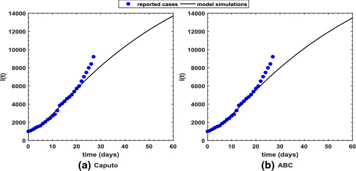
Fitting of parameters is one of the important features during validation of an epidemiological model. This creates confidence in the acceptance of the model in order to use it for future prediction and to better understand the transmission dynamics of the underlying epidemic. Thus, we aim to explain the fitting of parameters through least-squares curve fitting technique in this section. Since there are 19 different parameters in the proposed model for COVID-19 pandemic, we have estimated two of the parameters, whereas the rest are best fitted based upon the real cases of COVID-19 pandemic throughout Pakistan (source http://covid.gov.pk/stats/pakistan). Two demographic parameters are $\mathrm{\Lambda }$ (recruitment rate) and $\lambda$ (natural death rate) which have been estimated. The average natural mortality rate of a Pakistani is 66.5 years (source https://www.worldlifeexpectancy.com/pakistan-life-expectancy) so this yields $\lambda =1/(66.5\ast 365)$ per day. Further, the total population of Pakistan is 212.2M; it may be assumed that $\mathrm{\Lambda }/\lambda$, which is the limiting population when there is no existence of the pandemic. In this way, $\mathrm{\Lambda }=8.7424+03$ per day. Daily cases of the pandemic are considered from March 24 to April 20, 2020 during preparation of the research paper. As far as the initial conditions are concerned, the total population of Pakistan is taken to be $N(0)=212.2\text{M}$, the initial exposed and quarantined population is taken as $E(0)=8,000,000,Q(0)=6,000,000$ and this further assists us to determine remaining initial conditions for the other state variables with the help of the identity $N(0)=S(0)+E(0)+Q(0)+A(0)+I(0)+P(0)+T(0)+R(0)$. In this connection, we have obtained $S(0)=194,198,880$, $A(0)=4,000,000$, $I(0)=1000$, $P(0)=0$, $T(0)=100$ and $R(0)=20.$ There are 19 biological parameters which have been estimated with the aid of least-square fitting method and this leads to yield a best fit of the proposed COVID-19 model’s solution to the actual cases of the pandemic as shown in Fig. 1. The average absolute relative error between COVID-19 actual cases and the model’s solution for the infectious class is tried to be reduced and the best fitted values of the relevant parameters have been achieved. Such a value for the error is approximately $6.6801e-02$. Figure 1 shows the real COVID-19 cases by blue solid circles, whereas the best fitted curve of the model is shown by the black solid line. The biological parameters included in the model are listed in Table 1 along with their best estimated values obtained via least-squares technique. These parameters have finally produced the value of the basic reproduction number equivalent to ${\mathcal{R}}_0=2.1828$ for the real COVID-19 cases in Pakistan from March 24 to April 20, 2020.

Fig. 1.

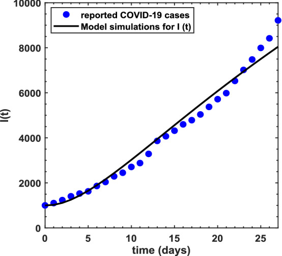
The daily COVID-19 cases time series in Pakistan from March 24 to April 20, 2020, and the best fitted curve from the proposed model

Table 1.

Estimated and best fitted values of the parameters used in the proposed COVID-19 model

Parameter	Meaning	Value	Sources
$\mathrm{\Lambda }$	Recruitment rate	$8.7424e+03$	Estimated
$\lambda$	Natural death rate	$1/(66.5\ast 365)$	Estimated
${\mu }_Q$	Modification factor for quarantined	0.124	Fitted
${\mu }_A$	Modification factor for asymptomatic	0.956	Fitted
${\mu }_P$	Modification factor for isolated	0.076	Fitted
$\rho$	Rate of joining treatment class	0.2	Fitted
$\sigma$	Diseases induced mortality rate	$1e-03$	Fitted
k	Proportion of asymptomatic individuals	$1e-04$	Fitted
${\beta }_1$	Recovery rate from quarantined individuals	0.0000005539	Fitted
${\beta }_2$	Recovery rate from asymptomatic individuals	0.0000000196	Fitted
${\beta }_3$	Recovery rate from symptomatic individuals	0.0000001257	Fitted
${\beta }_4$	Recovery rate from isolated individuals	0.0000001086	Fitted
${\beta }_5$	Recovery rate from treated individuals	0.6461299316	Fitted
$\delta$	Transmission rate	0.7925264407	Fitted
${\alpha }_1$	Rate at which the exposed individuals are diminished by quarantine	0.0000000032	Fitted
${\alpha }_2$	Rate at which the symptomatic individuals are diminished by isolation	0.0000001257	Fitted
$r_1$	Rate at which exposed become infected	0.0000230757	Fitted
$r_2$	Rate at which quarantined individuals are isolated	0.0000076749	Fitted
$\gamma$	Rate at which infected individuals are treated	0.0010169510	Fitted

Numerical scheme for the Caputo fractional COVID-19 model

This section of the paper focuses on the numerical simulation for the Caputo-type fractional-order coronavirus model in Eq. (12). The Adams-type predictor–corrector method [71–73, 80] that is used to achieve numerical simulation of the nonlinear system is proposed to obtain approximate solution of the mentioned model. The following form of Cauchy ordinary differential equation is considered with respect to the Caputo operator of order $\vartheta$:

$$\begin{array}{c}\hfill {}_0^C{D}_t^{\vartheta }\phi \left(t\right)=\mathrm{\Phi }\left(t,,,\phi ,\left(t\right)\right),{\phi }^{\left(p\right)}\left(0\right)={\phi }_0^p,0<\upsilon \le 1,0<t\le \tau ,\end{array}$$ 31

where $p=0,1,\dots ,n-1,n=⌈\vartheta ⌉$. Equation (31) can be converted to the following Volterra equation:

$$\begin{array}{c}\hfill \phi \left(t\right)=\sum _{p=0}^{n-1}{\phi }_0^{\left(p\right)}\frac{t^p}{p!}+\frac{1}{\mathrm{\Gamma }\left(\alpha \right)}{\int }_0^t{\left(t,-,s\right)}^{\alpha -1}\mathrm{\Phi }\left(s,,,\phi ,\left(s\right)\right)ds.\end{array}$$ 32

By using this mentioned predictor–corrector scheme associated with the Adam–Bashforth–Moulton algorithm [72] to get the numerical solutions of the fractional coronavirus model, we can take $h=\tau /N,t_j=jh,$ and $j=0,1,\dots ,N\in {\mathrm{Z}}^{+},$ by letting ${\phi }_j\approx \phi \left(t_j\right),$ it can be discretized as follows, i.e., the corresponding corrector formula [74]

$$\begin{array}{cc}\hfill S_{k+1}=& \sum _{j=0}^{k-1}{S}_0^{\left(j\right)}\frac{t_{k+1}^j}{j!}+\frac{h^{\vartheta }}{\mathrm{\Gamma }\left(\vartheta ,+,2\right)}\sum _{j=0}^k\left(q_{j,k+1}\right)\hfill \\ \hfill & \times \left(\mathrm{\Lambda },-,\frac{S_j\left(\delta ,I_j,+,{\mu }_Q,\delta ,Q_j,+,{\mu }_A,\delta ,A_j,+,{\mu }_P,\delta ,P_j\right)}{N-Q_j-P_j},-,\lambda ,S_j\right)\hfill \\ \hfill & +\frac{h^{\vartheta }}{\mathrm{\Gamma }\left(\vartheta ,+,2\right)}\sum _{j=0}^k\left(q_{k+1,k+1}\right)\hfill \\ \hfill & \times \left(\mathrm{\Lambda },-,\frac{S_{k+1}^{\mathit{PR}}\left(\delta ,I_{k+1}^{\mathit{PR}},+,{\mu }_Q,\delta ,Q_{k+1}^{\mathit{PR}},+,{\mu }_A,\delta ,A_{k+1}^{\mathit{PR}},+,{\mu }_P,\delta ,P_{k+1}^{\mathit{PR}}\right)}{N-Q_{k+1}^{\mathit{PR}}-Q_{k+1}^{\mathit{PR}}},-,\lambda ,S_{k+1}^{\mathit{PR}}\right),\hfill \\ \hfill E_{k+1}=& \sum _{j=0}^{k-1}{E}_0^{\left(j\right)}\frac{t_{k+1}^j}{j!}+\frac{h^{\vartheta }}{\mathrm{\Gamma }\left(\vartheta ,+,2\right)}\sum _{j=0}^k\left(q_{j,k+1}\right)\hfill \\ \hfill & \times \left(\frac{S_j\left(\delta ,I_j,+,{\mu }_Q,\delta ,Q_j,+,{\mu }_A,\delta ,A_j,+,{\mu }_P,\delta ,P_j\right)}{N-Q_j-P_j},-,\left({\alpha }_1,+,r_1,+,\lambda \right),E_j\right)\hfill \\ \hfill & +\frac{h^{\vartheta }}{\mathrm{\Gamma }\left(\vartheta ,+,2\right)}\sum _{j=0}^k\left(q_{k+1,k+1}\right)\hfill \\ \hfill & \times \left(\frac{S_{k+1}^{\mathit{PR}}\left(\delta ,I_{k+1}^{\mathit{PR}},+,{\mu }_Q,\delta ,Q_{k+1}^{\mathit{PR}},+,{\mu }_A,\delta ,A_{k+1}^{\mathit{PR}},+,{\mu }_P,\delta ,P_{k+1}^{\mathit{PR}}\right)}{N-Q_{k+1}^{\mathit{PR}}-Q_{k+1}^{\mathit{PR}}},-,\left({\alpha }_1,+,r_1,+,\lambda \right),E_{k+1}^{\mathit{PR}}\right),\hfill \\ \hfill Q_{k+1}=& \sum _{j=0}^{k-1}{Q}_0^{\left(j\right)}\frac{t_{k+1}^j}{j!}+\frac{h^{\vartheta }}{\mathrm{\Gamma }\left(\vartheta ,+,2\right)}\sum _{j=0}^k\left(q_{j,k+1}\right)\left({\alpha }_1,E_j,-,\left(r_2,+,{\beta }_1,+,\lambda \right),Q_j\right)\hfill \\ \hfill & +\frac{h^{\vartheta }}{\mathrm{\Gamma }\left(\vartheta ,+,2\right)}\sum _{j=0}^k\left(q_{k+1,k+1}\right)\left({\alpha }_1,E_{k+1}^{\mathit{PR}},-,\left(r_2,+,{\beta }_1,+,\lambda \right),Q_{k+1}^{\mathit{PR}}\right),\hfill \\ \hfill A_{k+1}=& \sum _{j=0}^{k-1}{A}_0^{\left(j\right)}\frac{t_{k+1}^j}{j!}+\frac{1}{\mathrm{\Gamma }\left(\vartheta \right)}\sum _{j=0}^k\left(q_{j,k+1}\right)\left(k,r_1,E_j,-,\left({\beta }_2,+,\lambda \right),A_j\right)\hfill \\ \hfill & +\frac{1}{\mathrm{\Gamma }\left(\vartheta \right)}\sum _{j=0}^k\left(q_{k+1,k+1}\right)\left(k,r_1,E_{k+1}^{\mathit{PR}},-,\left({\beta }_2,+,\lambda \right),A_{k+1}^{\mathit{PR}}\right),\hfill \\ \hfill I_{k+1}=& \sum _{j=0}^{k-1}{I}_0^{\left(j\right)}\frac{t_{k+1}^j}{j!}+\frac{h^{\vartheta }}{\mathrm{\Gamma }\left(\vartheta ,+,2\right)}\sum _{j=0}^k\left(q_{j,k+1}\right)\left(\left(1,-,k\right),r_1,E_j,-,\left({\alpha }_2,+,{\beta }_3,+,\rho ,+,\lambda \right),I_j\right)\hfill \\ \hfill & +\frac{h^{\vartheta }}{\mathrm{\Gamma }\left(\vartheta ,+,2\right)}\sum _{j=0}^k\left(q_{k+1,k+1}\right)\left(\left(1,-,k\right),r_1,E_{k+1}^{\mathit{PR}},-,\left({\alpha }_2,+,{\beta }_3,+,\rho ,+,\lambda \right),I_{k+1}^{\mathit{PR}}\right),\hfill \\ \hfill P_{k+1}=& \sum _{j=0}^{k-1}{P}_0^{\left(j\right)}\frac{t_{k+1}^j}{j!}+\frac{h^{\vartheta }}{\mathrm{\Gamma }\left(\vartheta ,+,2\right)}\sum _{j=0}^k\left(q_{j,k+1}\right)\left(r_2,Q_j,+,{\alpha }_2,I_j,-,\left(\sigma ,+,{\beta }_4,+,\lambda \right),P_j\right)\hfill \\ \hfill & +\frac{h^{\vartheta }}{\mathrm{\Gamma }\left(\vartheta ,+,2\right)}\sum _{j=0}^k\left(q_{k+1,k+1}\right)\left(r_2,Q_{k+1}^{\mathit{PR}},+,{\alpha }_2,I_{k+1}^{\mathit{PR}},-,\left(\sigma ,+,{\beta }_4,+,\lambda \right),P_{k+1}^{\mathit{PR}}\right),\hfill \\ \hfill T_{k+1}=& \sum _{j=0}^{k-1}{T}_0^{\left(j\right)}\frac{t_{k+1}^j}{j!}+\frac{h^{\vartheta }}{\mathrm{\Gamma }\left(\vartheta ,+,2\right)}\sum _{j=0}^k\left(q_{j,k+1}\right)\left(\gamma ,I_j,-,\left(\lambda ,+,{\beta }_5\right),T_j\right)\hfill \\ \hfill & +\frac{h^{\vartheta }}{\mathrm{\Gamma }\left(\vartheta ,+,2\right)}\sum _{j=0}^k\left(q_{k+1,k+1}\right)\left(\gamma ,I_{k+1}^{\mathit{PR}},-,\left(\lambda ,+,{\beta }_5\right),T_{k+1}^{\mathit{PR}}\right),\hfill \\ \hfill R_{k+1}=& \sum _{j=0}^{k-1}{R}_0^{\left(j\right)}\frac{t_{k+1}^j}{j!}+\frac{h^{\vartheta }}{\mathrm{\Gamma }\left(\vartheta ,+,2\right)}\sum _{j=0}^k\left(q_{j,k+1}\right)\hfill \\ \hfill & \times \left({\beta }_1,Q_j,+,{\beta }_2,A_j,+,{\beta }_3,I_j,+,{\beta }_4,P_j,+,{\beta }_5,T_j,-,\lambda ,R_j\right)\hfill \\ \hfill & +\frac{h^{\vartheta }}{\mathrm{\Gamma }\left(\vartheta ,+,2\right)}\sum _{j=0}^k\left(q_{k+1,k+1}\right)\hfill \\ \hfill & \times \left({\beta }_1,Q_{k+1}^{\mathit{PR}},+,{\beta }_2,A_{k+1}^{\mathit{PR}},+,{\beta }_3,I_{k+1}^{\mathit{PR}},+,{\beta }_4,P_{k+1}^{\mathit{PR}},+,{\beta }_5,T_{k+1}^{\mathit{PR}},-,\lambda ,R_{k+1}^{\mathit{PR}}\right),\hfill \end{array}$$

where

$$\begin{array}{c}\hfill q_{j,k+1}=\left\{\begin{array}{cc}{k}^{\vartheta +1}-\left(k,-,\vartheta \right){\left(k,+,1\right)}^{\vartheta },\hfill & \mathrm{if}j=0,\hfill \\ {\left(k,-,j,+,2\right)}^{\vartheta +1}+{\left(k,-,j\right)}^{\vartheta +1}-2{\left(k,-,j,+,1\right)}^{\vartheta +1},\hfill & \mathrm{if}1\le j\le k,\hfill \\ 1,\hfill & \mathrm{if}j=k+1.\hfill \end{array}\right)\end{array}$$ 33

Then, the required step is to determine the corresponding predictor formula ${\phi }_{k+1}^{\mathit{PR}}.$ We can calculate the mentioned predictor formula as

$$\begin{array}{cc}\hfill S_{k+1}^{\mathit{PR}}=& \sum _{j=0}^{k-1}{S}_0^{\left(j\right)}\frac{t_{k+1}^j}{j!}+\frac{h^{\vartheta }}{\mathrm{\Gamma }\left(\vartheta ,+,1\right)}\sum _{j=0}^k\left(z_{j,k+1}\right)\hfill \\ \hfill & \times \left(\mathrm{\Lambda },-,\frac{S_j\left(\delta ,I_j,+,{\mu }_Q,\delta ,Q_j,+,{\mu }_A,\delta ,A_j,+,{\mu }_P,\delta ,P_j\right)}{N-Q_j-P_j},-,\lambda ,S_j\right),\hfill \\ \hfill E_{k+1}^{\mathit{PR}}=& \sum _{j=0}^{k-1}{E}_0^{\left(j\right)}\frac{t_{k+1}^j}{j!}+\frac{h^{\vartheta }}{\mathrm{\Gamma }\left(\vartheta ,+,1\right)}\sum _{j=0}^k\left(z_{j,k+1}\right)\hfill \\ \hfill & \times \left(\frac{S_j\left(\delta ,I_j,+,{\mu }_Q,\delta ,Q_j,+,{\mu }_A,\delta ,A_j,+,{\mu }_P,\delta ,P_j\right)}{N-Q_j-P_j},-,\left({\alpha }_1,+,r_1,+,\lambda \right),E_j\right),\hfill \\ \hfill Q_{k+1}^{\mathit{PR}}=& \sum _{j=0}^{k-1}{Q}_0^{\left(j\right)}\frac{t_{k+1}^j}{j!}+\frac{h^{\vartheta }}{\mathrm{\Gamma }\left(\vartheta ,+,1\right)}\sum _{j=0}^k\left(z_{j,k+1}\right)\left({\alpha }_1,E_j,-,\left(r_2,+,{\beta }_1,+,\lambda \right),Q_j\right),\hfill \\ \hfill A_{k+1}^{\mathit{PR}}=& \sum _{j=0}^{k-1}{A}_0^{\left(j\right)}\frac{t_{k+1}^j}{j!}+\frac{h^{\vartheta }}{\mathrm{\Gamma }\left(\vartheta ,+,1\right)}\sum _{j=0}^k\left(z_{j,k+1}\right)\left(k,r_1,E_j,-,\left({\beta }_2,+,\lambda \right),A_j\right),\hfill \\ \hfill I_{k+1}^{\mathit{PR}}=& \sum _{j=0}^{k-1}{I}_0^{\left(j\right)}\frac{t_{k+1}^j}{j!}+\frac{h^{\vartheta }}{\mathrm{\Gamma }\left(\vartheta ,+,1\right)}\sum _{j=0}^k\left(z_{j,k+1}\right)\left(\left(1,-,k\right),r_1,E_j,-,\left({\alpha }_2,+,{\beta }_3,+,\rho ,+,\lambda \right),I_j\right),\hfill \\ \hfill P_{k+1}^{\mathit{PR}}=& \sum _{j=0}^{k-1}{P}_0^{\left(j\right)}\frac{t_{k+1}^j}{j!}+\frac{h^{\vartheta }}{\mathrm{\Gamma }\left(\vartheta ,+,1\right)}\sum _{j=0}^k\left(z_{j,k+1}\right)\left(r_2,Q_j,+,{\alpha }_2,I_j,-,\left(\sigma ,+,{\beta }_4,+,\lambda \right),P_j\right),\hfill \\ \hfill T_{k+1}^{\mathit{PR}}=& \sum _{j=0}^{k-1}{T}_0^{\left(j\right)}\frac{t_{k+1}^j}{j!}+\frac{h^{\vartheta }}{\mathrm{\Gamma }\left(\vartheta ,+,1\right)}\sum _{j=0}^k\left(z_{j,k+1}\right)\left(\gamma ,I_j,-,\left(\lambda ,+,{\beta }_5\right),T_j\right),\hfill \\ \hfill R_{k+1}^{\mathit{PR}}=& \sum _{j=0}^{k-1}{R}_0^{\left(j\right)}\frac{t_{k+1}^j}{j!}+\frac{h^{\vartheta }}{\mathrm{\Gamma }\left(\vartheta ,+,1\right)}\sum _{j=0}^k\hfill \\ \hfill & \left(z_{j,k+1}\right)\left({\beta }_1,Q_j,+,{\beta }_2,A_j,+,{\beta }_3,I_j,+,{\beta }_4,P_j,+,{\beta }_5,T_j,-,\lambda ,R_j\right),\hfill \end{array}$$

where

$$\begin{array}{c}\hfill z_{j,k+1}={\left(k,+,1,-,j\right)}^{\vartheta }-{\left(k,-,j\right)}^{\vartheta }.\end{array}$$

Numerical scheme for the ABC fractional COVID-19 model

In this section, the proposed COVID-19 epidemic model under the ABC fractional derivative of order $\vartheta$ is numerically simulated [79]. The method is used to obtain approximate solutions of the proposed model. To provide the estimated solution by means of this algorithm, the following nonlinear fractional differential equation with respect to the ABC fractional derivative of order $\vartheta$:

$$\begin{array}{c}\hfill {{}_0^{\mathrm{ABC}}D}_t^{\vartheta }\phi (t)=\Psi (t,\phi (t)),0\le t\le \tau \end{array}$$ 34

with the following initial conditions

$$\begin{array}{c}\hfill {\phi }^{\left(v\right)}\left(0\right)={\phi }_0^v,v=0,1,2,\dots ,[\vartheta ]-1.\end{array}$$ 35

Applying the fundamental theorem of fractional calculus, Eq. (34) can be converted to a fractional integral equation as

$$\begin{array}{c}\hfill \phi \left(t\right)-\phi \left(0\right)=\frac{\left(1,-,\vartheta \right)}{\aleph (\vartheta )}\Psi (t,\phi (t))+\frac{\vartheta }{\mathrm{\Gamma }(\vartheta )\aleph (\vartheta )}{\int }_0^t{(t-t)}^{\vartheta -1}\Psi (t,\phi (t))dt.\end{array}$$ 36

At a given point $t_{n+1}$, $n=0,1,2\cdots ,$ we have from Eq. (36)

$$\begin{array}{cc}\hfill \phi \left(t_{n+1}\right)-\phi \left(0\right)=& \frac{\left(1,-,\vartheta \right)}{\aleph (\vartheta )}\Psi (t_n,\phi (t_n))+\frac{\vartheta }{\aleph (\vartheta )\mathrm{\Gamma }(\vartheta )}{\int }_0^{t_{n+1}}{(t_{n+1}-t)}^{\vartheta -1}\Psi (\tau ,\phi (\tau ))d\tau ,\hfill \\ \hfill =& \frac{\left(1,-,\vartheta \right)}{\aleph (\vartheta )}\Psi (t_n,\phi (t_n))\hfill \\ \hfill & +\frac{\vartheta }{\aleph (\vartheta )\mathrm{\Gamma }(\vartheta )}\sum _{k=0}^n{\int }_{t_k}^{t_{k+1}}{(t_{n+1}-t)}^{\vartheta -1}\Psi (\tau ,\phi (\tau ))d\tau .\hfill \end{array}$$ 37

Within the interval $\left[t_k,,,t_{k+1}\right]$, the function $\Psi \left(\tau ,,,\phi ,\left(\tau \right)\right)$, using the two-step Lagrange polynomial interpolation, can be approximated as follows:

$$\begin{array}{cc}\hfill Z_k\left(\tau \right)=& \frac{\tau -t_{k-1}}{t_k-t_{k-1}}\Psi \left(t_k,,,\phi ,\left(t_k\right)\right)-\frac{\tau -t_k}{t_k-t_{k-1}}\Psi \left(t_{k-1},,,\phi ,\left(t_{k-1}\right)\right)\hfill \\ \hfill =& \frac{\Psi \left(t_k,,,\phi ,\left(t_k\right)\right)}{h}\left(\tau ,-,t_{k-1}\right)-\frac{\Psi \left(t_{k-1},,,\phi ,\left(t_{k-1}\right)\right)}{h}\left(\tau ,-,t_k\right)\hfill \\ \hfill \cong & \frac{\Psi \left(t_k,,,{\phi }_k\right)}{h}\left(\tau ,-,t_{k-1}\right)-\frac{\Psi \left(t_{k-1},,,,{\phi }_{k-1}\right)}{h}\left(\tau ,-,t_k\right).\hfill \end{array}$$ 38

Under the approximation Eq.(38), we get from Eq.(37) as

$$\begin{array}{cc}\hfill {\phi }_{n+1}=& \phi \left(0\right)+\frac{\left(1,-,\vartheta \right)}{\aleph \left(\vartheta \right)}\Psi \left(t_n,,,\phi ,\left(t_n\right)\right)+\frac{\vartheta }{\aleph \left(\vartheta \right)\times \mathrm{\Gamma }\left(\vartheta \right)}\hfill \\ \hfill & \times \sum _{k=0}^n\left(\frac{\Psi \left(t_k,,,{\phi }_k\right)}{h},{\int }_{t_k}^{t_{k+1}},({\tau -t}_{k-1},),{(t_{n+1}-t)}^{\vartheta -1},d,\tau \right)\hfill \\ \hfill & \left(-,\frac{\Psi \left(t_{k-1},,,{\phi }_{k-1}\right)}{h},{\int }_{t_k}^{t_{k+1}},({\tau -t}_k),{(t_{n+1}-t)}^{\vartheta -1},d,\tau \right).\hfill \end{array}$$ 39

Without loss of generality, we consider

$$\begin{array}{c}\hfill G_{\vartheta ,k,1}={\int }_{t_k}^{t_{k+1}}({\tau -t}_{k-1}){(t_{n+1}-t)}^{\vartheta -1}d\tau ,\end{array}$$

and

$$\begin{array}{c}\hfill G_{\vartheta ,k,2}={\int }_{t_k}^{t_{k+1}}({\tau -t}_k){(t_{n+1}-t)}^{\vartheta -1}d\tau .\end{array}$$

Therefore,

$$\begin{array}{c}\hfill G_{\vartheta ,k,1}=h^{\vartheta +1}\frac{{\left(n,+,1,-,k\right)}^{\vartheta }\left(n,-,k,+,2,+,\vartheta \right)-{\left(n,-,k\right)}^{\vartheta }\left(n,-,k,+,2,+,2,\vartheta \right)}{\vartheta \left(\vartheta ,+,1\right)},\end{array}$$ 40

and

$$\begin{array}{c}\hfill G_{\vartheta ,k,2}=h^{\vartheta +1}\frac{{\left(n,+,1,-,k\right)}^{\vartheta +1}-{\left(n,-,k\right)}^{\vartheta }\left(n,-,k,+,1,+,\vartheta \right)}{\vartheta \left(\vartheta ,+,1\right)}.\end{array}$$ 41

This implies from Eq. (39) after substituting Eqs. (40)–(41),

$$\begin{array}{cc}\hfill {\phi }_{n+1}=& \phi \left(0\right)+\frac{\left(1,-,\vartheta \right)}{\aleph \left(\vartheta \right)}\Psi \left(t_n,,,\phi ,\left(t_n\right)\right)+\frac{\vartheta }{\aleph \left(\vartheta \right)}\sum _{k=0}^n\hfill \\ \hfill & \times \left(\frac{h^{\vartheta }\Psi \left(t_k,,,{\phi }_k\right)}{\mathrm{\Gamma }\left(\vartheta ,+,2\right)},{(\left(n,+,1,-,k\right)}^{\vartheta },\left(n,-,k,+,2,+,\vartheta \right),-,{\left(n,-,k\right)}^{\vartheta },\left(n,-,k,+,2,+,2,\vartheta \right),)\right)\hfill \\ \hfill & -\frac{\vartheta }{\aleph \left(\vartheta \right)}\sum _{k=0}^n\left(\frac{h^{\vartheta }\Psi \left(t_{k-1},,,{\phi }_{k-1}\right)}{\mathrm{\Gamma }\left(\vartheta ,+,2\right)},{(\left(n,+,1,-,k\right)}^{\vartheta +1},-,{\left(n,-,k\right)}^{\vartheta },\left(n,-,k,+,1,+,\vartheta \right),)\right).\hfill \\ \hfill \end{array}$$ 42

Equation (42) gives the numerical scheme for Atangana–Baleanu fractional derivative in the sense of Caputo. Using this scheme for the numerical solutions of the proposed fractional coronavirus model, we get

$$\begin{array}{cc}\hfill S_{n+1}=& S\left(0\right)+\frac{\left(1,-,\vartheta \right)}{\aleph \left(\vartheta \right)}\Psi \left(t_n,,,S,\left(t_n\right)\right)+\frac{\vartheta }{\aleph \left(\vartheta \right)}\sum _{k=0}^n\hfill \\ \hfill & \times \left(\frac{h^{\vartheta }\Psi \left(t_k,,,S_k\right)}{\mathrm{\Gamma }\left(\vartheta ,+,2\right)},{(\left(n,+,1,-,k\right)}^{\vartheta },\left(n,-,k,+,2,+,\vartheta \right),-,{\left(n,-,k\right)}^{\vartheta },\left(n,-,k,+,2,+,2,\vartheta \right),)\right)\hfill \\ \hfill & -\frac{\vartheta }{\aleph \left(\vartheta \right)}\sum _{k=0}^n\left(\frac{h^{\vartheta }\Psi \left(t_{k-1},,,S_{k-1}\right)}{\mathrm{\Gamma }\left(\vartheta ,+,2\right)},{(\left(n,+,1,-,k\right)}^{\vartheta +1},-,{\left(n,-,k\right)}^{\vartheta },\left(n,-,k,+,1,+,\vartheta \right),)\right),\hfill \\ \hfill E_{n+1}=& E\left(0\right)+\frac{\left(1,-,\vartheta \right)}{\aleph \left(\vartheta \right)}\Psi \left(t_n,,,E,\left(t_n\right)\right)+\frac{\vartheta }{\aleph \left(\vartheta \right)}\sum _{k=0}^n\hfill \\ \hfill & \times \left(\frac{h^{\vartheta }\Psi \left(t_k,,,E_k\right)}{\mathrm{\Gamma }\left(\vartheta ,+,2\right)},{(\left(n,+,1,-,k\right)}^{\vartheta },\left(n,-,k,+,2,+,\vartheta \right),-,{\left(n,-,k\right)}^{\vartheta },\left(n,-,k,+,2,+,2,\vartheta \right),)\right)\hfill \\ \hfill & -\frac{\vartheta }{\aleph \left(\vartheta \right)}\sum _{k=0}^n\left(\frac{h^{\vartheta }\Psi \left(t_{k-1},,,E_{k-1}\right)}{\mathrm{\Gamma }\left(\vartheta ,+,2\right)},{(\left(n,+,1,-,k\right)}^{\vartheta +1},-,{\left(n,-,k\right)}^{\vartheta },\left(n,-,k,+,1,+,\vartheta \right),)\right),\hfill \\ \hfill Q_{n+1}=& Q\left(0\right)+\frac{\left(1,-,\vartheta \right)}{\aleph \left(\vartheta \right)}\Psi \left(t_n,,,Q,\left(t_n\right)\right)+\frac{\vartheta }{\aleph \left(\vartheta \right)}\sum _{k=0}^n\hfill \\ \hfill & \times \left(\frac{h^{\vartheta }\Psi \left(t_k,,,Q_k\right)}{\mathrm{\Gamma }\left(\vartheta ,+,2\right)},{(\left(n,+,1,-,k\right)}^{\vartheta },\left(n,-,k,+,2,+,\vartheta \right),-,{\left(n,-,k\right)}^{\vartheta },\left(n,-,k,+,2,+,2,\vartheta \right),)\right)\hfill \\ \hfill & -\frac{\vartheta }{\aleph \left(\vartheta \right)}\sum _{k=0}^n\left(\frac{h^{\vartheta }\Psi \left(t_{k-1},,,Q_{k-1}\right)}{\mathrm{\Gamma }\left(\vartheta ,+,2\right)},{(\left(n,+,1,-,k\right)}^{\vartheta +1},-,{\left(n,-,k\right)}^{\vartheta },\left(n,-,k,+,1,+,\vartheta \right),)\right),\hfill \\ \hfill A_{n+1}=& A\left(0\right)+\frac{\left(1,-,\vartheta \right)}{\aleph \left(\vartheta \right)}\Psi \left(t_n,,,A,\left(t_n\right)\right)+\frac{\vartheta }{\aleph \left(\vartheta \right)}\sum _{k=0}^n\hfill \\ \hfill & \times \left(\frac{h^{\vartheta }\Psi \left(t_k,,,A_k\right)}{\mathrm{\Gamma }\left(\vartheta ,+,2\right)},{(\left(n,+,1,-,k\right)}^{\vartheta },\left(n,-,k,+,2,+,\vartheta \right),-,{\left(n,-,k\right)}^{\vartheta },\left(n,-,k,+,2,+,2,\vartheta \right),)\right)\hfill \\ \hfill & -\frac{\vartheta }{\aleph \left(\vartheta \right)}\sum _{k=0}^n\left(\frac{h^{\vartheta }\Psi \left(t_{k-1},,,A_{k-1}\right)}{\mathrm{\Gamma }\left(\vartheta ,+,2\right)},{(\left(n,+,1,-,k\right)}^{\vartheta +1},-,{\left(n,-,k\right)}^{\vartheta },\left(n,-,k,+,1,+,\vartheta \right),)\right),\hfill \\ \hfill I_{n+1}=& I\left(0\right)+\frac{\left(1,-,\vartheta \right)}{\aleph \left(\vartheta \right)}\Psi \left(t_n,,,I,\left(t_n\right)\right)+\frac{\vartheta }{\aleph \left(\vartheta \right)}\sum _{k=0}^n\hfill \\ \hfill & \times \left(\frac{h^{\vartheta }\Psi \left(t_k,,,I_k\right)}{\mathrm{\Gamma }\left(\vartheta ,+,2\right)},{(\left(n,+,1,-,k\right)}^{\vartheta },\left(n,-,k,+,2,+,\vartheta \right),-,{\left(n,-,k\right)}^{\vartheta },\left(n,-,k,+,2,+,2,\vartheta \right),)\right)\hfill \\ \hfill & -\frac{\vartheta }{\aleph \left(\vartheta \right)}\sum _{k=0}^n\left(\frac{h^{\vartheta }\Psi \left(t_{k-1},,,I_{k-1}\right)}{\mathrm{\Gamma }\left(\vartheta ,+,2\right)},{(\left(n,+,1,-,k\right)}^{\vartheta +1},-,{\left(n,-,k\right)}^{\vartheta },\left(n,-,k,+,1,+,\vartheta \right),)\right),\hfill \\ \hfill P_{n+1}=& P\left(0\right)+\frac{\left(1,-,\vartheta \right)}{\aleph \left(\vartheta \right)}\Psi \left(t_n,,,P,\left(t_n\right)\right)+\frac{\vartheta }{\aleph \left(\vartheta \right)}\sum _{k=0}^n\hfill \\ \hfill & \times \left(\frac{h^{\vartheta }\Psi \left(t_k,,,P_k\right)}{\mathrm{\Gamma }\left(\vartheta ,+,2\right)},{(\left(n,+,1,-,k\right)}^{\vartheta },\left(n,-,k,+,2,+,\vartheta \right),-,{\left(n,-,k\right)}^{\vartheta },\left(n,-,k,+,2,+,2,\vartheta \right),)\right)\hfill \\ \hfill & -\frac{\vartheta }{\aleph \left(\vartheta \right)}\sum _{k=0}^n\left(\frac{h^{\vartheta }\Psi \left(t_{k-1},,,P_{k-1}\right)}{\mathrm{\Gamma }\left(\vartheta ,+,2\right)},{(\left(n,+,1,-,k\right)}^{\vartheta +1},-,{\left(n,-,k\right)}^{\vartheta },\left(n,-,k,+,1,+,\vartheta \right),)\right),\hfill \\ \hfill T_{n+1}=& T\left(0\right)+\frac{\left(1,-,\vartheta \right)}{\aleph \left(\vartheta \right)}\Psi \left(t_n,,,T,\left(t_n\right)\right)+\frac{\vartheta }{\aleph \left(\vartheta \right)}\sum _{k=0}^n\hfill \\ \hfill & \times \left(\frac{h^{\vartheta }\Psi \left(t_k,,,T_k\right)}{\mathrm{\Gamma }\left(\vartheta ,+,2\right)},{(\left(n,+,1,-,k\right)}^{\vartheta },\left(n,-,k,+,2,+,\vartheta \right),-,{\left(n,-,k\right)}^{\vartheta },\left(n,-,k,+,2,+,2,\vartheta \right),)\right)\hfill \\ \hfill & -\frac{\vartheta }{\aleph \left(\vartheta \right)}\sum _{k=0}^n\left(\frac{h^{\vartheta }\Psi \left(t_{k-1},,,T_{k-1}\right)}{\mathrm{\Gamma }\left(\vartheta ,+,2\right)},{(\left(n,+,1,-,k\right)}^{\vartheta +1},-,{\left(n,-,k\right)}^{\vartheta },\left(n,-,k,+,1,+,\vartheta \right),)\right),\hfill \\ \hfill R_{n+1}=& R\left(0\right)+\frac{\left(1,-,\vartheta \right)}{\aleph \left(\vartheta \right)}\Psi \left(t_n,,,R,\left(t_n\right)\right)+\frac{\vartheta }{\aleph \left(\vartheta \right)}\sum _{k=0}^n\hfill \\ \hfill & \times \left(\frac{h^{\vartheta }\Psi \left(t_k,,,R_k\right)}{\mathrm{\Gamma }\left(\vartheta ,+,2\right)},{(\left(n,+,1,-,k\right)}^{\vartheta },\left(n,-,k,+,2,+,\vartheta \right),-,{\left(n,-,k\right)}^{\vartheta },\left(n,-,k,+,2,+,2,\vartheta \right),)\right)\hfill \\ \hfill & -\frac{\vartheta }{\aleph \left(\vartheta \right)}\sum _{k=0}^n\left(\frac{h^{\vartheta }\Psi \left(t_{k-1},,,R_{k-1}\right)}{\mathrm{\Gamma }\left(\vartheta ,+,2\right)},{(\left(n,+,1,-,k\right)}^{\vartheta +1},-,{\left(n,-,k\right)}^{\vartheta },\left(n,-,k,+,1,+,\vartheta \right),)\right),\hfill \end{array}$$

Numerical simulations and discussion

In this section, we have investigated behavior of each state variable of the proposed COVID-19 model under the two fractional-order operators called the Caputo (having singular kernel) and Atangana–Baleanu–Caputo (having non-singular kernel). Profiles for the state variables have been graphically obtained based upon variation in the fractional-order parameter $\vartheta$ and the variation in some of the more important biological parameters of the model randomly taken from Table 1. In addition to this, 3D meshes and contour plots are shown to capture behavior of the basic reproduction number ${\mathcal{R}}_0$ in order to better understand the transmission dynamics of the pandemic.

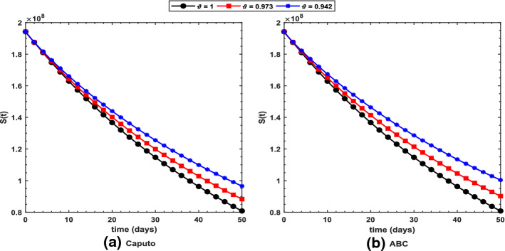
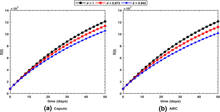
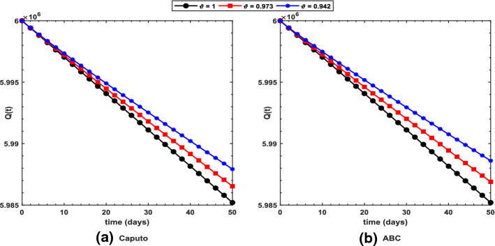
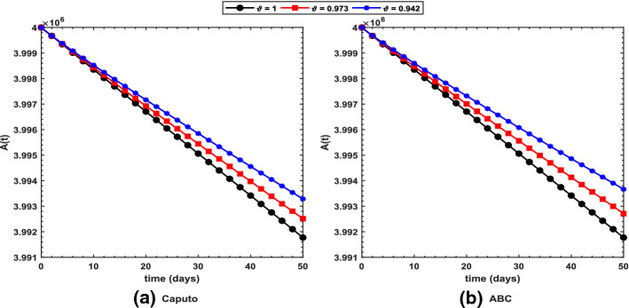
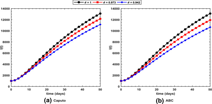
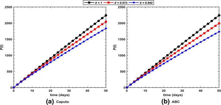
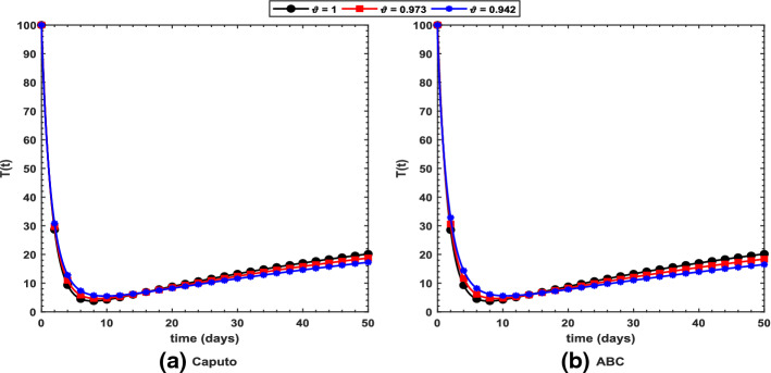
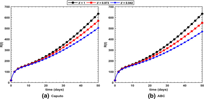
Figure 2 shows long-term behavior of the pandemic using the Caputo and the ABC operators. It has been observed that at the end of 60 days, the total number of symptomatic individuals would reach about $1.372e+04$ under the Caputo operator, whereas this number gets $1.348e+04$ for the ABC operator. Thus, ABC predicts about 240 more infectious cases in comparison with the prediction obtained under the Caputo operator. This seems to be in good agreement with the ongoing situation of this pandemic. We have shown dynamical behavior of each state variable from the proposed COVID-19 model in Figs. 3, 4, 5, 6, 7, 8, 9 and 10 for varying values of the fractional-order parameter $\vartheta$. Figure 3 shows increasing behavior of the susceptible population for decreasing values of $\vartheta$ with ABC operator predicting more susceptibility. Similar sort of behavior is observed in quarantined and asymptomatic population as depicted in Figs. 5 and 6, respectively. However, a different kind of behavior exists for rest of the state variables of the model. Figure 7 depicts significance of the fractional-order parameter $\vartheta$ for the symptomatic population of the model. This plot shows substantial decrease in the number of infectious individuals for decreasing values of $\vartheta$ under both operators with Caputo predicting 490 more cases in comparison with ABC operator assuming $\vartheta =0.942$. For behavior of isolated population, Fig. 8 depicts that for decreasing values of $\vartheta$ in both operators, the number of isolated individuals decreases with 102 more people isolated in case of Caputo when $\vartheta =0.942$. Under the treatment profile, Caputo operator predicts one extra case as shown in Fig. 9 for $\vartheta =0.942$. Further, the Caputo operator suggests that 34 more symptomatic cases get recovered with $\vartheta =0.942$ in comparison with ABC operator. However, we observed previously that the Caputo generates 490 additional infectious cases. Thus, the ABC gives better agreement with real situation in this regard.

Fig. 2.

Long-term prediction for infectious population in Pakistan using the proposed COVID-19 model under the a Caputo and b ABC operators with $\vartheta =0.973$

Fig. 3.

Profile for the susceptible population using the proposed COVID-19 model under the a Caputo and b ABC operators with different values of $\vartheta$

Fig. 4.

Profile for the exposed population using the proposed COVID-19 model under the a Caputo and b ABC operators with different values of $\vartheta$

Fig. 5.

Profile for the quarantined population using the proposed COVID-19 model under the a Caputo and b ABC operators with different values of $\vartheta$

Fig. 6.

Profile for the asymptomatic population using the proposed COVID-19 model under the a Caputo and b ABC operators with different values of $\vartheta$

Fig. 7.

Profile for the symptomatic population using the proposed COVID-19 model under the a Caputo and b ABC operators with different values of $\vartheta$

Fig. 8.

Profile for the isolated population using the proposed COVID-19 model under the a Caputo and b ABC operators with different values of $\vartheta$

Fig. 9.

Profile for the treated population using the proposed COVID-19 model under the a Caputo and b ABC operators with different values of $\vartheta$

Fig. 10.

Profile for the recovered population using the proposed COVID-19 model under the a Caputo and b ABC operators with different values of $\vartheta$

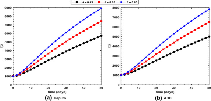
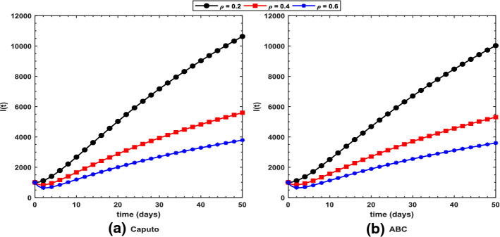
It can be observed from Fig. 11 that for increasing values of $\delta$ (transmission rate), the symptomatic individuals increase under both operators with Caputo predicting 8923 cases, whereas ABC predicts 7840 cases for $\delta =0.85$ at the end of the chosen time interval, thereby recommending the use of ABC operator over the Caputo. Increasing values of $\rho$ (rate of joining treatment class) result in decreasing number of symptomatic individuals as depicted in Fig. 12. For $\rho =0.6$, Caputo in Fig. 12a predicts 3789 symptomatic cases, whereas ABC in Fig. 12b suggests 3600 cases demonstrating effectiveness of ABC operator over the Caputo.

Fig. 11.

Profile for the symptomatic I(t) population using the proposed COVID-19 model under the a Caputo and b ABC operators with different values of $\delta$ (transmission rate) while taking $\vartheta =0.853$

Fig. 12.

Profile for the symptomatic I(t) population using the proposed COVID-19 model under the a Caputo and b ABC operators with different values of $\rho$ (rate of joining treatment class) while taking $\vartheta =0.926$

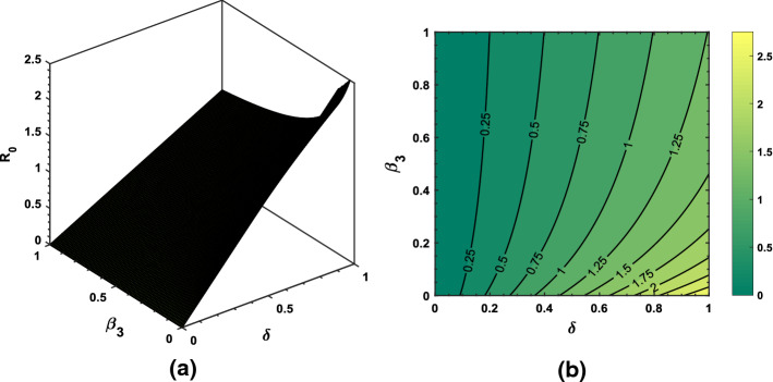
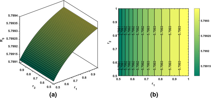
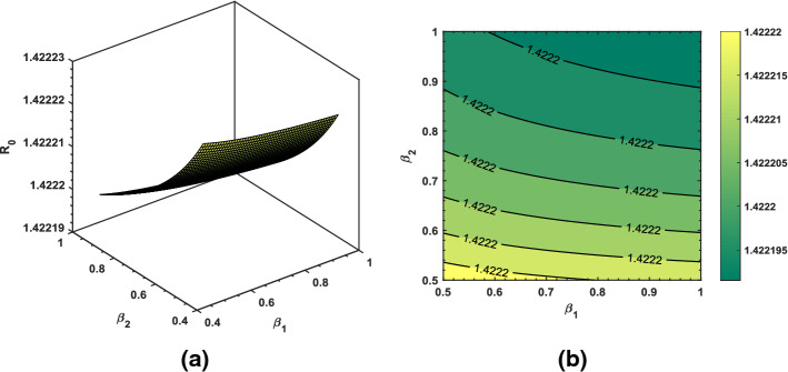
Using some randomly chosen parameters from Table 1, we have shown transmission behavior of the pandemic via basic reproduction number ${\mathcal{R}}_0$. As shown in Fig. 13, increasing $\delta$ and decreasing ${\beta }_3$ will produce ${\mathcal{R}}_0$ greater than 2 which is an alarming sign. Thus, reducing transmission rate of the coronavirus is the most essential strategy in order to prevent the virus further spread. Similar sort of behavior and description of the associated ${\mathcal{R}}_0$ in Figs. 14 and 15 can be interpreted based upon the biological parameters used for the analysis.

Fig. 13.

Dynamical behavior of the basic reproduction number $R_0$ for varying values of $\delta$ (transmission rate) and ${\beta }_3$ (recovery rate from symptomatic class)

Fig. 14.

Dynamical behavior of the basic reproduction number $R_0$ for varying values of $r_1$ (rate at which exposed become infected) and $r_2$ (rate at which quarantined are isolated)

Fig. 15.

Dynamical behavior of the basic reproduction number $R_0$ for varying values of ${\beta }_1$ (recovery rate from quarantined class) and ${\beta }_2$ (recovery rate from asymptomatic class)

Conclusions

In this paper, modeling and analysis of the newly emerged coronavirus (COVID-19) transmission dynamics have been provided in fractional-order derivatives with treatment class for the infected population. The basic reproduction number ${\mathcal{R}}_0$ has been computed by the next-generation matrix method which performs as a threshold parameter in the disease transmission and determines whether the disease persists or vanishes from the population. The positivity and boundedness of the solutions have been determined. Also, the stability conditions of the equilibrium points for the proposed fractional-order system have been discussed. Meanwhile, the global dynamics of the equilibria has been obtained by the Lyapunov functional approach method. Based on the mathematical analysis, the disease-free equilibrium is locally asymptotically stable when ${\mathcal{R}}_0<1$ that means the infection will die out in the population. On the other hand, the infection spreads in the population when ${\mathcal{R}}_0>1.$ Numerically, the endemic equilibrium tends to be locally asymptotically stable when ${\mathcal{R}}_0>1$, which means that the infection will persist in the population. Moreover, the fitting of parameters through least-squares curve fitting technique has been done and the average absolute relative error between COVID-19 actual cases and the model’s solution for the infectious class is tried to be reduced, and the best fitted values of the relevant parameters have been achieved. Finally, Adams–Bashforth–Moulton method has been applied to carry out the numerical simulations for different values of the fractional-order $\vartheta$ of the proposed model. It has been demonstrated that physical processes are better well described using the derivatives of fractional order which are more accurate and reliable in comparison with the classical-order case. Hence, we replace the integer-order time derivative with the Caputo-type fractional-order derivative and Atangana–Baleanu fractional-order derivative. It has been shown that these operators have many advantages over the existing non-integer-order types. Our choice of using the Caputo and Atangana–Baleanu derivatives is because they allow traditional initial and boundary conditions to be included in the formulation of the problem. We have formulated the model based on the available information we gathered on media and in prints about the causative agent and model of transmission of the virus disease. A number of numerical results showing the behavior of the dynamics obtained for different instances of fractional-order have been reported.

Although the fractional-order COVID-19 epidemic model based upon Caputo and ABC operators provides sufficient information to understand the epidemic transmission process and help to determine the crucial factors for its spread, for more detailed analysis one needs to have new tools to disclose unnoticed behavior of such nonlinear epidemiological systems and thus the operators known as Caputo–Fabrizio, Atangana–Gomez, Atangana beta derivative, truncated M-derivative, fractal–fractional and others can be used in future research work. In addition to this, our future research would also devise new strategies for carrying out stability analysis of the epidemiological models based upon non-autonomous nonlinear ordinary differential equations with fractional-order derivatives.

Appendix

The coefficients in Eq. (25) are given as

$$\begin{array}{cc}\hfill {\lambda }_1=& K^2\left({\alpha }_1,+,{\alpha }_2,+,{\beta }_1,+,{\beta }_2,+,{\beta }_3,+,{\beta }_4,+,6,\lambda ,+,r_1,+,r_2,+,\rho ,+,\sigma \right)+KM,\hfill \\ \hfill {\lambda }_2=& 15K^2{\lambda }^2+KM{\alpha }_1+KM{\alpha }_2+KM{\beta }_1+KM{\beta }_2+KM{\beta }_3+KM{\beta }_4\hfill \\ \hfill & -MS{\alpha }_1+5KM\lambda +KM{r}_1+KM{r}_2+KM\rho +KM\sigma +K^2{\alpha }_1{\alpha }_2+K^2{\alpha }_1{\beta }_1\hfill \\ \hfill & +K^2{\alpha }_1{\beta }_2+K^2{\alpha }_2{\beta }_1+K^2{\alpha }_1{\beta }_3\hfill \\ \hfill & +K^2{\alpha }_2{\beta }_2+K^2{\alpha }_1{\beta }_4+K^2{\alpha }_2{\beta }_4+K^2{\beta }_1{\beta }_2+K^2{\beta }_1{\beta }_3+K^2{\beta }_1{\beta }_4+K^2{\beta }_2{\beta }_3\hfill \\ \hfill & +K^2{\beta }_2{\beta }_4+K^2{\beta }_3{\beta }_4+5K^2{\alpha }_1\lambda +5K^2{\alpha }_2\lambda +5K^2{\beta }_1\lambda +5K^2{\beta }_2\lambda +5K^2{\beta }_3\lambda \hfill \\ \hfill & +5K^2{\beta }_4\lambda +K^2{\alpha }_1{r}_2+K^2{\alpha }_2{r}_1+K^2{\alpha }_2{r}_2+K^2{\alpha }_1\rho +K^2{\beta }_1{r}_1\hfill \\ \hfill & +K^2{\beta }_2{r}_1+K^2{\beta }_2{r}_2+K^2{\beta }_3{r}_1+K^2{\beta }_3{r}_2+K^2{\beta }_4{r}_1+K^2{\beta }_4{r}_2\hfill \\ \hfill & +K^2{\beta }_1\rho +K^2{\beta }_2\rho +K^2{\beta }_4\rho +K^2{\alpha }_1\sigma +K^2{\alpha }_2\sigma +K^2{\beta }_1\sigma \hfill \\ \hfill & +K^2{\beta }_2\sigma +K^2{\beta }_3\sigma +5K^2\lambda r_1\hfill \\ \hfill & +5K^2\lambda r_2+5K^2\lambda \rho +5K^2\lambda \sigma +K^2{r}_1{r}_2+K^2{r}_1\rho +K^2{r}_2\rho \hfill \\ \hfill & +K^2{r}_1\sigma +K^2{r}_2\sigma +K^2\rho \sigma -KS\delta r_1-KS{\alpha }_1\delta {\mu }_Q+KS\delta k{r}_1-KS\delta k{\mu }_A{r}_1,\hfill \\ \hfill {\lambda }_3=& 20K^2{\lambda }^3+10K^2{\alpha }_1{\lambda }^2+10K^2{\alpha }_2{\lambda }^2+10K^2{\beta }_1{\lambda }^2\hfill \\ \hfill & +10K^2{\beta }_2{\lambda }^2+10K^2{\beta }_3{\lambda }^2+10K^2{\beta }_4{\lambda }^2+10K^2{\lambda }^2{r}_1+10K^2{\lambda }^2{r}_2\hfill \\ \hfill & +10K^2{\lambda }^2\rho +10K^2{\lambda }^2\sigma +10KM{\lambda }^2+K^2{\alpha }_1{\alpha }_2{\beta }_1\hfill \\ \hfill & +K^2{\alpha }_1{\alpha }_2{\beta }_2+K^2{\alpha }_1{\alpha }_2{\beta }_4+K^2{\alpha }_1{\beta }_1{\beta }_2+K^2{\alpha }_1{\beta }_1{\beta }_3\hfill \\ \hfill & +K^2{\alpha }_2{\beta }_1{\beta }_2+K^2{\alpha }_1{\beta }_1{\beta }_4+K^2{\alpha }_1{\beta }_2{\beta }_3\hfill \\ \hfill & +K^2{\alpha }_1{\beta }_2{\beta }_4+K^2{\alpha }_2{\beta }_1{\beta }_4+K^2{\alpha }_1{\beta }_3{\beta }_4+K^2{\alpha }_2{\beta }_2{\beta }_4\hfill \\ \hfill & +K^2{\beta }_1{\beta }_2{\beta }_3+K^2{\beta }_1{\beta }_2{\beta }_4+K^2{\beta }_1{\beta }_3{\beta }_4\hfill \\ \hfill \end{array}$$

$$\begin{array}{cc}& +K^2{\beta }_2{\beta }_3{\beta }_4+4K^2{\alpha }_1{\alpha }_2\lambda +4K^2{\alpha }_1{\beta }_1\lambda +4K^2{\alpha }_1{\beta }_2\lambda \hfill \\ \hfill & +4K^2{\alpha }_2{\beta }_1\lambda +4K^2{\alpha }_1{\beta }_3\lambda +4K^2{\alpha }_2{\beta }_2\lambda \hfill \\ \hfill & +4K^2{\alpha }_1{\beta }_4\lambda +4K^2{\alpha }_2{\beta }_4\lambda +4K^2{\beta }_1{\beta }_2\lambda +4K^2{\beta }_1{\beta }_3\lambda \hfill \\ \hfill & +4K^2{\beta }_1{\beta }_4\lambda +4K^2{\beta }_2{\beta }_3\lambda +4K^2{\beta }_2{\beta }_4\lambda \hfill \\ \hfill & +4K^2{\beta }_3{\beta }_4\lambda +K^2{\alpha }_1{\alpha }_2{r}_2+K^2{\alpha }_2{\beta }_1{r}_1+K^2{\alpha }_1{\beta }_2{r}_2\hfill \\ \hfill & +K^2{\alpha }_2{\beta }_2{r}_1+K^2{\alpha }_1{\beta }_3{r}_2+K^2{\alpha }_2{\beta }_2{r}_2+K^2{\alpha }_1{\beta }_4{r}_2\hfill \\ \hfill & +K^2{\alpha }_2{\beta }_4{r}_1+K^2{\alpha }_2{\beta }_4{r}_2+K^2{\alpha }_1{\beta }_1\rho +K^2{\alpha }_1{\beta }_2\rho \hfill \\ \hfill & +K^2{\alpha }_1{\beta }_4\rho +K^2{\alpha }_1{\alpha }_2\sigma +K^2{\beta }_1{\beta }_2{r}_1+K^2{\beta }_1{\beta }_3{r}_1\hfill \\ \hfill & +K^2{\beta }_1{\beta }_4{r}_1+K^2{\beta }_2{\beta }_3{r}_1+K^2{\beta }_2{\beta }_3{r}_2+K^2{\beta }_2{\beta }_4{r}_1\hfill \\ \hfill & +K^2{\beta }_2{\beta }_4{r}_2+K^2{\beta }_3{\beta }_4{r}_1+K^2{\beta }_3{\beta }_4{r}_2+K^2{\beta }_1{\beta }_2\rho \hfill \\ \hfill & +K^2{\beta }_1{\beta }_4\rho +K^2{\beta }_2{\beta }_4\rho +K^2{\alpha }_1{\beta }_1\sigma +K^2{\alpha }_1{\beta }_2\sigma \hfill \\ \hfill & +K^2{\alpha }_2{\beta }_1\sigma +K^2{\alpha }_1{\beta }_3\sigma +K^2{\alpha }_2{\beta }_2\sigma +K^2{\beta }_1{\beta }_2\sigma \hfill \\ \hfill & +K^2{\beta }_1{\beta }_3\sigma +K^2{\beta }_2{\beta }_3\sigma +4K^2{\alpha }_1\lambda r_2+4K^2{\alpha }_2\lambda r_1+4K^2{\alpha }_2\lambda r_2\hfill \\ \hfill & +4K^2{\alpha }_1\lambda \rho +4K^2{\beta }_1\lambda r_1+4K^2{\beta }_2\lambda r_1+4K^2{\beta }_2\lambda r_2\hfill \\ \hfill & +4K^2{\beta }_3\lambda r_1+4K^2{\beta }_3\lambda r_2+4K^2{\beta }_4\lambda r_1+4K^2{\beta }_4\lambda r_2\hfill \\ \hfill & +4K^2{\beta }_1\lambda \rho +4K^2{\beta }_2\lambda \rho +4K^2{\beta }_4\lambda \rho +4K^2{\alpha }_1\lambda \sigma \hfill \\ \hfill & +4K^2{\alpha }_2\lambda \sigma +4K^2{\beta }_1\lambda \sigma +4K^2{\beta }_2\lambda \sigma +4K^2{\beta }_3\lambda \sigma \hfill \\ \hfill & +K^2{\alpha }_2{r}_1{r}_2+K^2{\alpha }_1{r}_2\rho +K^2{\beta }_2{r}_1{r}_2+K^2{\beta }_3{r}_1{r}_2\hfill \\ \hfill & +K^2{\beta }_4{r}_1{r}_2+K^2{\beta }_1{r}_1\rho +K^2{\beta }_2{r}_1\rho +K^2{\beta }_2{r}_2\rho +K^2{\beta }_4{r}_1\rho \hfill \\ \hfill & +K^2{\beta }_4{r}_2\rho +K^2{\alpha }_1{r}_2\sigma +K^2{\alpha }_2{r}_1\sigma +K^2{\alpha }_2{r}_2\sigma \hfill \\ \hfill \end{array}$$

$$\begin{array}{cc}& +K^2{\alpha }_1\rho \sigma +K^2{\beta }_1{r}_1\sigma +K^2{\beta }_2{r}_1\sigma +K^2{\beta }_2{r}_2\sigma \hfill \\ \hfill & +K^2{\beta }_3{r}_1\sigma +K^2{\beta }_3{r}_2\sigma +K^2{\beta }_1\rho \sigma +K^2{\beta }_2\rho \sigma \hfill \\ \hfill & +4K^2\lambda r_1{r}_2+4K^2\lambda r_1\rho +4K^2\lambda r_2\rho +4K^2\lambda r_1\sigma \hfill \\ \hfill & +4K^2\lambda r_2\sigma +4K^2\lambda \rho \sigma +K^2{r}_1{r}_2\rho +K^2{r}_1{r}_2\sigma +K^2{r}_1\rho \sigma \hfill \\ \hfill & +K^2{r}_2\rho \sigma +KM{\alpha }_1{\alpha }_2+KM{\alpha }_1{\beta }_1+KM{\alpha }_1{\beta }_2\hfill \\ \hfill & +KM{\alpha }_2{\beta }_1+KM{\alpha }_1{\beta }_3+KM{\alpha }_2{\beta }_2+KM{\alpha }_1{\beta }_4+KM{\alpha }_2{\beta }_4+KM{\beta }_1{\beta }_2\hfill \\ \hfill & +KM{\beta }_1{\beta }_3+KM{\beta }_1{\beta }_4+KM{\beta }_2{\beta }_3+KM{\beta }_2{\beta }_4+KM{\beta }_3{\beta }_4\hfill \\ \hfill & -MS{\alpha }_1{\alpha }_2-MS{\alpha }_1{\beta }_2-MS{\alpha }_1{\beta }_3-MS{\alpha }_1{\beta }_4\hfill \\ \hfill & +4KM{\alpha }_1\lambda +4KM{\alpha }_2\lambda +4KM{\beta }_1\lambda +4KM{\beta }_2\lambda \hfill \\ \hfill & +4KM{\beta }_3\lambda +4KM{\beta }_4\lambda +KM{\alpha }_1{r}_2+KM{\alpha }_2{r}_1+KM{\alpha }_2{r}_2\hfill \\ \hfill & +KM{\alpha }_1\rho +KM{\beta }_1{r}_1+KM{\beta }_2{r}_1+KM{\beta }_2{r}_2+KM{\beta }_3{r}_1+KM{\beta }_3{r}_2\hfill \\ \hfill & +KM{\beta }_4{r}_1+KM{\beta }_4{r}_2+KM{\beta }_1\rho +KM{\beta }_2\rho +KM{\beta }_4\rho +KM{\alpha }_1\sigma \hfill \\ \hfill & +KM{\alpha }_2\sigma -4MS{\alpha }_1\lambda +KM{\beta }_1\sigma +KM{\beta }_2\sigma +KM{\beta }_3\sigma \hfill \\ \hfill & -MS{\alpha }_1{r}_2-MS{\alpha }_2{r}_1-MS{\alpha }_1\rho -MS{\alpha }_1\sigma +4KM\lambda r_1+4KM\lambda r_2\hfill \\ \hfill & +4KM\lambda \rho +4KM\lambda \sigma +KM{r}_1{r}_2+KM{r}_1\rho +KM{r}_2\rho +KM{r}_1\sigma \hfill \\ \hfill & +KM{r}_2\sigma +KM\rho \sigma -KS{\beta }_1\delta r_1-KS{\beta }_2\delta r_1-KS{\beta }_4\delta r_1\hfill \\ \hfill & +MS{\alpha }_{2}k{r}_1-4KS\delta \lambda r_1-KS\delta r_1{r}_2-KS\delta r_1\sigma \hfill \\ \hfill \end{array}$$

$$\begin{array}{cc}& -KS{\alpha }_1{\alpha }_2\delta {\mu }_Q-KS{\alpha }_1{\beta }_2\delta {\mu }_Q-KS{\alpha }_1{\beta }_3\delta {\mu }_Q\hfill \\ \hfill & -KS{\alpha }_1{\beta }_4\delta {\mu }_Q-4KS{\alpha }_1\delta \lambda {\mu }_Q+KS{\beta }_1\delta k{r}_1\hfill \\ \hfill & +KS{\beta }_2\delta k{r}_1+KS{\beta }_4\delta k{r}_1-KS{\alpha }_1\delta {\mu }_P{r}_2\hfill \\ \hfill & -KS{\alpha }_2\delta {\mu }_P{r}_1-KS{\alpha }_1\delta {\mu }_Q\rho -KS{\alpha }_1\delta {\mu }_Q\sigma \hfill \\ \hfill & +4KS\delta k\lambda r_1+KS\delta k{r}_1{r}_2+KS\delta k{r}_1\sigma -KS{\alpha }_2\delta k{\mu }_A{r}_1\hfill \\ \hfill & +KS{\alpha }_2\delta k{\mu }_P{r}_1-KS{\beta }_1\delta k{\mu }_A{r}_1-KS{\beta }_3\delta k{\mu }_A{r}_1\hfill \\ \hfill & -KS{\beta }_4\delta k{\mu }_A{r}_1-4KS\delta k\lambda {\mu }_A{r}_1-KS\delta k{\mu }_A{r}_1{r}_2\hfill \\ \hfill & -KS\delta k{\mu }_A{r}_1\rho -KS\delta k{\mu }_A{r}_1\sigma ,\hfill \\ \hfill {\lambda }_4=& 15K^2{\lambda }^4+10K^2{\alpha }_1{\lambda }^3+10K^2{\alpha }_2{\lambda }^3+10K^2{\beta }_1{\lambda }^3\hfill \\ \hfill & +10K^2{\beta }_2{\lambda }^3+10K^2{\beta }_3{\lambda }^3+10K^2{\beta }_4{\lambda }^3+10K^2{\lambda }^3{r}_1+10K^2{\lambda }^3{r}_2\hfill \\ \hfill & +10K^2{\lambda }^3\rho +10K^2{\lambda }^3\sigma +10KM{\lambda }^3+6KM{\alpha }_1{\lambda }^2\hfill \\ \hfill & +6KM{\alpha }_2{\lambda }^2+6KM{\beta }_1{\lambda }^2+6KM{\beta }_2{\lambda }^2+6KM{\beta }_3{\lambda }^2\hfill \\ \hfill & +6KM{\beta }_4{\lambda }^2-6MS{\alpha }_1{\lambda }^2+6KM{\lambda }^2{r}_1+6KM{\lambda }^2{r}_2\hfill \\ \hfill & +6KM{\lambda }^2\rho +6KM{\lambda }^2\sigma +6K^2{\alpha }_1{\alpha }_2{\lambda }^2+6K^2{\alpha }_1{\beta }_1{\lambda }^2\hfill \\ \hfill & +6K^2{\alpha }_1{\beta }_2{\lambda }^2+6K^2{\alpha }_2{\beta }_1{\lambda }^2+6K^2{\alpha }_1{\beta }_3{\lambda }^2\hfill \\ \hfill & +6K^2{\alpha }_2{\beta }_2{\lambda }^2+6K^2{\alpha }_1{\beta }_4{\lambda }^2+6K^2{\alpha }_2{\beta }_4{\lambda }^2\hfill \\ \hfill & +6K^2{\beta }_1{\beta }_2{\lambda }^2+6K^2{\beta }_1{\beta }_3{\lambda }^2+6K^2{\beta }_1{\beta }_4{\lambda }^2+6K^2{\beta }_2{\beta }_3{\lambda }^2\hfill \\ \hfill & +6K^2{\beta }_2{\beta }_4{\lambda }^2+6K^2{\beta }_3{\beta }_4{\lambda }^2+6K^2{\alpha }_1{\lambda }^2{r}_2+6K^2{\alpha }_2{\lambda }^2{r}_1\hfill \\ \hfill & +6K^2{\alpha }_2{\lambda }^2{r}_2+6K^2{\alpha }_1{\lambda }^2\rho +6K^2{\beta }_1{\lambda }^2{r}_1\hfill \\ \hfill \end{array}$$

$$\begin{array}{cc}& +6K^2{\beta }_2{\lambda }^2{r}_1+6K^2{\beta }_2{\lambda }^2{r}_2+6K^2{\beta }_3{\lambda }^2{r}_1+6K^2{\beta }_3{\lambda }^2{r}_2\hfill \\ \hfill & +6K^2{\beta }_4{\lambda }^2{r}_1+6K^2{\beta }_4{\lambda }^2{r}_2+6K^2{\beta }_1{\lambda }^2\rho \hfill \\ \hfill & +6K^2{\beta }_2{\lambda }^2\rho +6K^2{\beta }_4{\lambda }^2\rho +6K^2{\alpha }_1{\lambda }^2\sigma +6K^2{\alpha }_2{\lambda }^2\sigma \hfill \\ \hfill & +6K^2{\beta }_1{\lambda }^2\sigma +6K^2{\beta }_2{\lambda }^2\sigma +6K^2{\beta }_3{\lambda }^2\sigma \hfill \\ \hfill & +6K^2{\lambda }^2{r}_1{r}_2+6K^2{\lambda }^2{r}_1\rho +6K^2{\lambda }^2{r}_2\rho +6K^2{\lambda }^2{r}_1\sigma \hfill \\ \hfill & +6K^2{\lambda }^2{r}_2\sigma +6K^2{\lambda }^2\rho \sigma +KM{\alpha }_1{\alpha }_2{\beta }_1\hfill \\ \hfill & +KM{\alpha }_1{\alpha }_2{\beta }_2+KM{\alpha }_1{\alpha }_2{\beta }_4+KM{\alpha }_1{\beta }_1{\beta }_2+KM{\alpha }_1{\beta }_1{\beta }_3\hfill \\ \hfill & +KM{\alpha }_2{\beta }_1{\beta }_2+KM{\alpha }_1{\beta }_1{\beta }_4+KM{\alpha }_1{\beta }_2{\beta }_3\hfill \\ \hfill & +KM{\alpha }_1{\beta }_2{\beta }_4+KM{\alpha }_2{\beta }_1{\beta }_4+KM{\alpha }_1{\beta }_3{\beta }_4+KM{\alpha }_2{\beta }_2{\beta }_4\hfill \\ \hfill & +KM{\beta }_1{\beta }_2{\beta }_3+KM{\beta }_1{\beta }_2{\beta }_4+KM{\beta }_1{\beta }_3{\beta }_4\hfill \\ \hfill & +KM{\beta }_2{\beta }_3{\beta }_4-MS{\alpha }_1{\alpha }_2{\beta }_2-MS{\alpha }_1{\alpha }_2{\beta }_4\hfill \\ \hfill & -MS{\alpha }_1{\beta }_2{\beta }_3-MS{\alpha }_1{\beta }_2{\beta }_4-MS{\alpha }_1{\beta }_3{\beta }_4+3KM{\alpha }_1{\alpha }_2\lambda \hfill \\ \hfill & +3KM{\alpha }_1{\beta }_1\lambda +3KM{\alpha }_1{\beta }_2\lambda +3KM{\alpha }_2{\beta }_1\lambda \hfill \\ \hfill & +3KM{\alpha }_1{\beta }_3\lambda +3KM{\alpha }_2{\beta }_2\lambda +3KM{\alpha }_1{\beta }_4\lambda \hfill \\ \hfill & +3KM{\alpha }_2{\beta }_4\lambda +3KM{\beta }_1{\beta }_2\lambda +3KM{\beta }_1{\beta }_3\lambda +3KM{\beta }_1{\beta }_4\lambda \hfill \\ \hfill & +3KM{\beta }_2{\beta }_3\lambda +3KM{\beta }_2{\beta }_4\lambda +3KM{\beta }_3{\beta }_4\lambda \hfill \\ \hfill \end{array}$$

$$\begin{array}{cc}& +KM{\alpha }_1{\alpha }_2{r}_2+KM{\alpha }_2{\beta }_1{r}_1+KM{\alpha }_1{\beta }_2{r}_2+KM{\alpha }_2{\beta }_2{r}_1\hfill \\ \hfill & +KM{\alpha }_1{\beta }_3{r}_2+KM{\alpha }_2{\beta }_2{r}_2+KM{\alpha }_1{\beta }_4{r}_2+KM{\alpha }_2{\beta }_4{r}_1\hfill \\ \hfill & +KM{\alpha }_2{\beta }_4{r}_2+KM{\alpha }_1{\beta }_1\rho +KM{\alpha }_1{\beta }_2\rho +KM{\alpha }_1{\beta }_4\rho \hfill \\ \hfill & +KM{\alpha }_1{\alpha }_2\sigma +KM{\beta }_1{\beta }_2{r}_1+KM{\beta }_1{\beta }_3{r}_1+KM{\beta }_1{\beta }_4{r}_1\hfill \\ \hfill & +KM{\beta }_2{\beta }_3{r}_1+KM{\beta }_2{\beta }_3{r}_2+KM{\beta }_2{\beta }_4{r}_1+KM{\beta }_2{\beta }_4{r}_2\hfill \\ \hfill & +KM{\beta }_3{\beta }_4{r}_1+KM{\beta }_3{\beta }_4{r}_2+KM{\beta }_1{\beta }_2\rho +KM{\beta }_1{\beta }_4\rho \hfill \\ \hfill & +KM{\beta }_2{\beta }_4\rho -3MS{\alpha }_1{\alpha }_2\lambda +KM{\alpha }_1{\beta }_1\sigma +KM{\alpha }_1{\beta }_2\sigma \hfill \\ \hfill & +KM{\alpha }_2{\beta }_1\sigma +KM{\alpha }_1{\beta }_3\sigma +KM{\alpha }_2{\beta }_2\sigma -3MS{\alpha }_1{\beta }_2\lambda -3MS{\alpha }_1{\beta }_3\lambda \hfill \\ \hfill & -3MS{\alpha }_1{\beta }_4\lambda +KM{\beta }_1{\beta }_2\sigma +KM{\beta }_1{\beta }_3\sigma \hfill \\ \hfill & +KM{\beta }_2{\beta }_3\sigma -MS{\alpha }_1{\alpha }_2{r}_2-MS{\alpha }_2{\beta }_1{r}_1-MS{\alpha }_1{\beta }_2{r}_2\hfill \\ \hfill & -MS{\alpha }_2{\beta }_2{r}_1-MS{\alpha }_1{\beta }_3{r}_2-MS{\alpha }_1{\beta }_2\rho -MS{\alpha }_1{\beta }_4\rho \hfill \\ \hfill & -MS{\alpha }_1{\alpha }_2\sigma -MS{\alpha }_1{\beta }_2\sigma -MS{\alpha }_1{\beta }_3\sigma +3KM{\alpha }_1\lambda r_2\hfill \\ \hfill & +3KM{\alpha }_2\lambda r_1+3KM{\alpha }_2\lambda r_2+3KM{\alpha }_1\lambda \rho +3KM{\beta }_1\lambda r_1+3KM{\beta }_2\lambda r_1\hfill \\ \hfill & +3KM{\beta }_2\lambda r_2+3KM{\beta }_3\lambda r_1+3KM{\beta }_3\lambda r_2+3KM{\beta }_4\lambda r_1\hfill \\ \hfill & +3KM{\beta }_4\lambda r_2+3KM{\beta }_1\lambda \rho +3KM{\beta }_2\lambda \rho +3KM{\beta }_4\lambda \rho \hfill \\ \hfill & +3KM{\alpha }_1\lambda \sigma +3KM{\alpha }_2\lambda \sigma +3KM{\beta }_1\lambda \sigma \hfill \\ \hfill & +3KM{\beta }_2\lambda \sigma +3KM{\beta }_3\lambda \sigma +KM{\alpha }_2{r}_1{r}_2+KM{\alpha }_1{r}_2\rho \hfill \\ \hfill & +KM{\beta }_2{r}_1{r}_2+KM{\beta }_3{r}_1{r}_2+KM{\beta }_4{r}_1{r}_2+KM{\beta }_1{r}_1\rho \hfill \\ \hfill & +KM{\beta }_2{r}_1\rho +KM{\beta }_2{r}_2\rho +KM{\beta }_4{r}_1\rho +KM{\beta }_4{r}_2\rho \hfill \\ \hfill & +KM{\alpha }_1{r}_2\sigma +KM{\alpha }_2{r}_1\sigma +KM{\alpha }_2{r}_2\sigma +KM{\alpha }_1\rho \sigma \hfill \\ \hfill \end{array}$$

$$\begin{array}{cc}& -3MS{\alpha }_1\lambda r_2-3MS{\alpha }_2\lambda r_1+KM{\beta }_1{r}_1\sigma +KM{\beta }_2{r}_1\sigma \hfill \\ \hfill & +KM{\beta }_2{r}_2\sigma +KM{\beta }_3{r}_1\sigma +KM{\beta }_3{r}_2\sigma -3MS{\alpha }_1\lambda \rho \hfill \\ \hfill & +KM{\beta }_1\rho \sigma +KM{\beta }_2\rho \sigma -3MS{\alpha }_1\lambda \sigma -MS{\alpha }_2{r}_1{r}_2\hfill \\ \hfill & -MS{\alpha }_1{r}_2\rho -MS{\alpha }_1\rho \sigma +3KM\lambda r_1{r}_2+3KM\lambda r_1\rho \hfill \\ \hfill & +3KM\lambda r_2\rho +3KM\lambda r_1\sigma +3KM\lambda r_2\sigma +3KM\lambda \rho \sigma \hfill \\ \hfill & +KM{r}_1{r}_2\rho +KM{r}_1{r}_2\sigma +KM{r}_1\rho \sigma +KM{r}_2\rho \sigma +K^2{\alpha }_1{\alpha }_2{\beta }_1{\beta }_2\hfill \\ \hfill & +K^2{\alpha }_1{\alpha }_2{\beta }_1{\beta }_4+K^2{\alpha }_1{\alpha }_2{\beta }_2{\beta }_4\hfill \\ \hfill & +K^2{\alpha }_1{\beta }_1{\beta }_2{\beta }_3+K^2{\alpha }_1{\beta }_1{\beta }_2{\beta }_4+K^2{\alpha }_1{\beta }_1{\beta }_3{\beta }_4\hfill \\ \hfill & +K^2{\alpha }_2{\beta }_1{\beta }_2{\beta }_4+K^2{\alpha }_1{\beta }_2{\beta }_3{\beta }_4+K^2{\beta }_1{\beta }_2{\beta }_3{\beta }_4\hfill \\ \hfill & +3K^2{\alpha }_1{\alpha }_2{\beta }_1\lambda +3K^2{\alpha }_1{\alpha }_2{\beta }_2\lambda +3K^2{\alpha }_1{\alpha }_2{\beta }_4\lambda \hfill \\ \hfill & +3K^2{\alpha }_1{\beta }_1{\beta }_2\lambda +3K^2{\alpha }_1{\beta }_1{\beta }_3\lambda \hfill \\ \hfill & +3K^2{\alpha }_2{\beta }_1{\beta }_2\lambda +3K^2{\alpha }_1{\beta }_1{\beta }_4\lambda +3K^2{\alpha }_1{\beta }_2{\beta }_3\lambda \hfill \\ \hfill & +3K^2{\alpha }_1{\beta }_2{\beta }_4\lambda +3K^2{\alpha }_2{\beta }_1{\beta }_4\lambda +3K^2{\alpha }_1{\beta }_3{\beta }_4\lambda \hfill \\ \hfill & +3K^2{\alpha }_2{\beta }_2{\beta }_4\lambda +3K^2{\beta }_1{\beta }_2{\beta }_3\lambda +3K^2{\beta }_1{\beta }_2{\beta }_4\lambda \hfill \\ \hfill & +3K^2{\beta }_1{\beta }_3{\beta }_4\lambda +3K^2{\beta }_2{\beta }_3{\beta }_4\lambda -6KS\delta {\lambda }^2{r}_1\hfill \\ \hfill & +K^2{\alpha }_1{\alpha }_2{\beta }_2{r}_2+K^2{\alpha }_1{\alpha }_2{\beta }_4{r}_2+K^2{\alpha }_2{\beta }_1{\beta }_2{r}_1\hfill \\ \hfill & +K^2{\alpha }_1{\beta }_2{\beta }_3{r}_2+K^2{\alpha }_2{\beta }_1{\beta }_4{r}_1+K^2{\alpha }_1{\beta }_2{\beta }_4{r}_2\hfill \\ \hfill & +K^2{\alpha }_2{\beta }_2{\beta }_4{r}_1+K^2{\alpha }_1{\beta }_3{\beta }_4{r}_2+K^2{\alpha }_2{\beta }_2{\beta }_4{r}_2\hfill \\ \hfill & +K^2{\alpha }_1{\beta }_1{\beta }_2\rho +K^2{\alpha }_1{\beta }_1{\beta }_4\rho +K^2{\alpha }_1{\beta }_2{\beta }_4\rho \hfill \\ \hfill & +K^2{\alpha }_1{\alpha }_2{\beta }_1\sigma +K^2{\alpha }_1{\alpha }_2{\beta }_2\sigma +K^2{\beta }_1{\beta }_2{\beta }_3{r}_1\hfill \\ \hfill & +K^2{\beta }_1{\beta }_2{\beta }_4{r}_1+K^2{\beta }_1{\beta }_3{\beta }_4{r}_1+K^2{\beta }_2{\beta }_3{\beta }_4{r}_1\hfill \\ \hfill & +K^2{\beta }_2{\beta }_3{\beta }_4{r}_2+K^2{\beta }_1{\beta }_2{\beta }_4\rho +K^2{\alpha }_1{\beta }_1{\beta }_2\sigma \hfill \\ \hfill & +K^2{\alpha }_1{\beta }_1{\beta }_3\sigma +K^2{\alpha }_2{\beta }_1{\beta }_2\sigma +K^2{\alpha }_1{\beta }_2{\beta }_3\sigma \hfill \\ \hfill & +K^2{\beta }_1{\beta }_2{\beta }_3\sigma +3K^2{\alpha }_1{\alpha }_2\lambda r_2+3K^2{\alpha }_2{\beta }_1\lambda r_1\hfill \\ \hfill & +3K^2{\alpha }_1{\beta }_2\lambda r_2+3K^2{\alpha }_2{\beta }_2\lambda r_1\hfill \\ \hfill & +3K^2{\alpha }_1{\beta }_3\lambda r_2+3K^2{\alpha }_2{\beta }_2\lambda r_2+3K^2{\alpha }_1{\beta }_4\lambda r_2\hfill \\ \hfill & +3K^2{\alpha }_2{\beta }_4\lambda r_1+3K^2{\alpha }_2{\beta }_4\lambda r_2+3K^2{\alpha }_1{\beta }_1\lambda \rho \hfill \\ \hfill & +3K^2{\alpha }_1{\beta }_2\lambda \rho +3K^2{\alpha }_1{\beta }_4\lambda \rho +3K^2{\alpha }_1{\alpha }_2\lambda \sigma \hfill \\ \hfill & +3K^2{\beta }_1{\beta }_2\lambda r_1+3K^2{\beta }_1{\beta }_3\lambda r_1+3K^2{\beta }_1{\beta }_4\lambda r_1\hfill \\ \hfill & +3K^2{\beta }_2{\beta }_3\lambda r_1+3K^2{\beta }_2{\beta }_3\lambda r_2+3K^2{\beta }_2{\beta }_4\lambda r_1\hfill \\ \hfill & +3K^2{\beta }_2{\beta }_4\lambda r_2+3K^2{\beta }_3{\beta }_4\lambda r_1+3K^2{\beta }_3{\beta }_4\lambda r_2\hfill \\ \hfill & +3K^2{\beta }_1{\beta }_2\lambda \rho +3K^2{\beta }_1{\beta }_4\lambda \rho +3K^2{\beta }_2{\beta }_4\lambda \rho \hfill \\ \hfill & +3K^2{\alpha }_1{\beta }_1\lambda \sigma +3K^2{\alpha }_1{\beta }_2\lambda \sigma \hfill \\ \hfill & +3K^2{\alpha }_2{\beta }_1\lambda \sigma +3K^2{\alpha }_1{\beta }_3\lambda \sigma +3K^2{\alpha }_2{\beta }_2\lambda \sigma \hfill \\ \hfill & +3K^2{\beta }_1{\beta }_2\lambda \sigma +3K^2{\beta }_1{\beta }_3\lambda \sigma +3K^2{\beta }_2{\beta }_3\lambda \sigma \hfill \\ \hfill & +K^2{\alpha }_2{\beta }_2{r}_1{r}_2+K^2{\alpha }_2{\beta }_4{r}_1{r}_2+K^2{\alpha }_1{\beta }_2{r}_2\rho \hfill \\ \hfill & +K^2{\alpha }_1{\beta }_4{r}_2\rho +K^2{\alpha }_1{\alpha }_2{r}_2\sigma +K^2{\beta }_2{\beta }_3{r}_1{r}_2+K^2{\beta }_2{\beta }_4{r}_1{r}_2\hfill \\ \hfill & +K^2{\beta }_3{\beta }_4{r}_1{r}_2+K^2{\beta }_1{\beta }_2{r}_1\rho +K^2{\beta }_1{\beta }_4{r}_1\rho \hfill \\ \hfill \end{array}$$

$$\begin{array}{cc}& +K^2{\beta }_2{\beta }_4{r}_1\rho +K^2{\beta }_2{\beta }_4{r}_2\rho +K^2{\alpha }_2{\beta }_1{r}_1\sigma +K^2{\alpha }_1{\beta }_2{r}_2\sigma \hfill \\ \hfill & +K^2{\alpha }_2{\beta }_2{r}_1\sigma +K^2{\alpha }_1{\beta }_3{r}_2\sigma +K^2{\alpha }_2{\beta }_2{r}_2\sigma \hfill \\ \hfill & +K^2{\alpha }_1{\beta }_1\rho \sigma +K^2{\alpha }_1{\beta }_2\rho \sigma +K^2{\beta }_1{\beta }_2{r}_1\sigma \hfill \\ \hfill & +K^2{\beta }_1{\beta }_3{r}_1\sigma +K^2{\beta }_2{\beta }_3{r}_1\sigma +K^2{\beta }_2{\beta }_3{r}_2\sigma \hfill \\ \hfill & +K^2{\beta }_1{\beta }_2\rho \sigma +3K^2{\alpha }_2\lambda r_1{r}_2+3K^2{\alpha }_1\lambda r_2\rho +3K^2{\beta }_2\lambda r_1{r}_2\hfill \\ \hfill & +3K^2{\beta }_3\lambda r_1{r}_2+3K^2{\beta }_4\lambda r_1{r}_2+3K^2{\beta }_1\lambda r_1\rho \hfill \\ \hfill & +3K^2{\beta }_2\lambda r_1\rho +3K^2{\beta }_2\lambda r_2\rho +3K^2{\beta }_4\lambda r_1\rho \hfill \\ \hfill & +3K^2{\beta }_4\lambda r_2\rho +3K^2{\alpha }_1\lambda r_2\sigma +3K^2{\alpha }_2\lambda r_1\sigma \hfill \\ \hfill & +3K^2{\alpha }_2\lambda r_2\sigma +3K^2{\alpha }_1\lambda \rho \sigma +3K^2{\beta }_1\lambda r_1\sigma \hfill \\ \hfill & +3K^2{\beta }_2\lambda r_1\sigma +3K^2{\beta }_2\lambda r_2\sigma +3K^2{\beta }_3\lambda r_1\sigma \hfill \\ \hfill & +3K^2{\beta }_3\lambda r_2\sigma +3K^2{\beta }_1\lambda \rho \sigma +3K^2{\beta }_2\lambda \rho \sigma \hfill \\ \hfill & +K^2{\beta }_2{r}_1{r}_2\rho +K^2{\beta }_4{r}_1{r}_2\rho +K^2{\alpha }_2{r}_1{r}_2\sigma \hfill \\ \hfill & +K^2{\alpha }_1{r}_2\rho \sigma +K^2{\beta }_2{r}_1{r}_2\sigma +K^2{\beta }_3{r}_1{r}_2\sigma +K^2{\beta }_1{r}_1\rho \sigma \hfill \\ \hfill & +K^2{\beta }_2{r}_1\rho \sigma +K^2{\beta }_2{r}_2\rho \sigma +3K^2\lambda r_1{r}_2\rho +3K^2\lambda r_1{r}_2\sigma \hfill \\ \hfill & +3K^2\lambda r_1\rho \sigma +3K^2\lambda r_2\rho \sigma +K^2{r}_1{r}_2\rho \sigma \hfill \\ \hfill & +6KS\delta k{\lambda }^2{r}_1-KS{\beta }_1{\beta }_2\delta r_1-KS{\beta }_1{\beta }_4\delta r_1\hfill \\ \hfill & -KS{\beta }_2{\beta }_4\delta r_1+MS{\alpha }_2{\beta }_{1}k{r}_1+MS{\alpha }_2{\beta }_{2}k{r}_1-3KS{\beta }_1\delta \lambda r_1\hfill \\ \hfill & -3KS{\beta }_2\delta \lambda r_1-3KS{\beta }_4\delta \lambda r_1-KS{\beta }_2\delta r_1{r}_2\hfill \\ \hfill & -KS{\beta }_4\delta r_1{r}_2-KS{\beta }_1\delta r_1\sigma -KS{\beta }_2\delta r_1\sigma +3MS{\alpha }_{2}k\lambda r_1\hfill \\ \hfill & +MS{\alpha }_{2}k{r}_1{r}_2-3KS\delta \lambda r_1{r}_2-3KS\delta \lambda r_1\sigma -KS\delta r_1{r}_2\sigma \hfill \\ \hfill & -6KS{\alpha }_1\delta {\lambda }^2{\mu }_Q+KS{\beta }_1{\beta }_2\delta k{r}_1+KS{\beta }_1{\beta }_4\delta k{r}_1\hfill \\ \hfill & +KS{\beta }_2{\beta }_4\delta k{r}_1-KS{\alpha }_1{\alpha }_2\delta {\mu }_P{r}_2-KS{\alpha }_2{\beta }_1\delta {\mu }_P{r}_1\hfill \\ \hfill & -KS{\alpha }_1{\beta }_2\delta {\mu }_P{r}_2-KS{\alpha }_2{\beta }_2\delta {\mu }_P{r}_1-KS{\alpha }_1{\beta }_3\delta {\mu }_P{r}_2\hfill \\ \hfill & -KS{\alpha }_1{\beta }_2\delta {\mu }_Q\rho -KS{\alpha }_1{\beta }_4\delta {\mu }_Q\rho \hfill \\ \hfill & -KS{\alpha }_1{\alpha }_2\delta {\mu }_Q\sigma -KS{\alpha }_1{\beta }_2\delta {\mu }_Q\sigma -KS{\alpha }_1{\beta }_3\delta {\mu }_Q\sigma \hfill \\ \hfill & +3KS{\beta }_1\delta k\lambda r_1+3KS{\beta }_2\delta k\lambda r_1+3KS{\beta }_4\delta k\lambda r_1\hfill \\ \hfill & -3KS{\alpha }_1\delta \lambda {\mu }_P{r}_2-3KS{\alpha }_2\delta \lambda {\mu }_P{r}_1\hfill \\ \hfill & -3KS{\alpha }_1\delta \lambda {\mu }_Q\rho -3KS{\alpha }_1\delta \lambda {\mu }_Q\sigma \hfill \\ \hfill & +KS{\beta }_2\delta k{r}_1{r}_2+KS{\beta }_4\delta k{r}_1{r}_2+KS{\beta }_1\delta k{r}_1\sigma \hfill \\ \hfill & +KS{\beta }_2\delta k{r}_1\sigma -KS{\alpha }_2\delta {\mu }_P{r}_1{r}_2-KS{\alpha }_1\delta {\mu }_P{r}_2\rho \hfill \\ \hfill & -KS{\alpha }_1\delta {\mu }_Q\rho \sigma +3KS\delta k\lambda r_1{r}_2+3KS\delta k\lambda r_1\sigma \hfill \\ \hfill & +KS\delta k{r}_1{r}_2\sigma -6KS\delta k{\lambda }^2{\mu }_A{r}_1-KS{\alpha }_1{\alpha }_2{\beta }_2\delta {\mu }_Q\hfill \\ \hfill & -KS{\alpha }_1{\alpha }_2{\beta }_4\delta {\mu }_Q-KS{\alpha }_1{\beta }_2{\beta }_3\delta {\mu }_Q\hfill \\ \hfill & -KS{\alpha }_1{\beta }_2{\beta }_4\delta {\mu }_Q-KS{\alpha }_1{\beta }_3{\beta }_4\delta {\mu }_Q-3KS{\alpha }_1{\alpha }_2\delta \lambda {\mu }_Q\hfill \\ \hfill & -3KS{\alpha }_1{\beta }_2\delta \lambda {\mu }_Q-3KS{\alpha }_1{\beta }_3\delta \lambda {\mu }_Q\hfill \\ \hfill & -3KS{\alpha }_1{\beta }_4\delta \lambda {\mu }_Q-KS{\alpha }_2{\beta }_1\delta k{\mu }_A{r}_1\hfill \\ \hfill & -KS{\alpha }_2{\beta }_4\delta k{\mu }_A{r}_1+KS{\alpha }_2{\beta }_1\delta k{\mu }_P{r}_1+KS{\alpha }_2{\beta }_2\delta k{\mu }_P{r}_1\hfill \\ \hfill & -KS{\beta }_1{\beta }_3\delta k{\mu }_A{r}_1-KS{\beta }_1{\beta }_4\delta k{\mu }_A{r}_1\hfill \\ \hfill & -KS{\beta }_3{\beta }_4\delta k{\mu }_A{r}_1-3KS{\alpha }_2\delta k\lambda {\mu }_A{r}_1+3KS{\alpha }_2\delta k\lambda {\mu }_P{r}_1\hfill \\ \hfill & -3KS{\beta }_1\delta k\lambda {\mu }_A{r}_1-3KS{\beta }_3\delta k\lambda {\mu }_A{r}_1\hfill \\ \hfill & -3KS{\beta }_4\delta k\lambda {\mu }_A{r}_1-KS{\alpha }_2\delta k{\mu }_A{r}_1{r}_2\hfill \\ \hfill & +KS{\alpha }_2\delta k{\mu }_P{r}_1{r}_2-KS{\beta }_3\delta k{\mu }_A{r}_1{r}_2-KS{\beta }_4\delta k{\mu }_A{r}_1{r}_2\hfill \\ \hfill & -KS{\beta }_1\delta k{\mu }_A{r}_1\rho -KS{\beta }_4\delta k{\mu }_A{r}_1\rho -KS{\alpha }_2\delta k{\mu }_A{r}_1\sigma \hfill \\ \hfill & -KS{\beta }_1\delta k{\mu }_A{r}_1\sigma -KS{\beta }_3\delta k{\mu }_A{r}_1\sigma \hfill \\ \hfill & -3KS\delta k\lambda {\mu }_A{r}_1{r}_2-3KS\delta k\lambda {\mu }_A{r}_1\rho -3KS\delta k\lambda {\mu }_A{r}_1\sigma \hfill \\ \hfill & -KS\delta k{\mu }_A{r}_1{r}_2\rho -KS\delta k{\mu }_A{r}_1{r}_2\sigma -KS\delta k{\mu }_A{r}_1\rho \sigma .\hfill \end{array}$$

Compliance with ethical standards

Conflicts of interest

The authors declare that they have no conflicts of interest to report regarding the present study.

References

- 1.https://www.who.int/emergencies/diseases/novel-coronavirus-2019/situation-reports. Date of Access: 05.02.2020
- 2.Zu J, Li ML, Li ZF, Shen MW, Xiao YN, Ji FP. Transmission patterns of COVID-19 in the mainland of China and the efficacy of different control strategies: a data- and model-driven study. Infect. Dis. Poverty. 2020;9:83. doi: 10.1186/s40249-020-00709-z. [DOI] [PMC free article] [PubMed] [Google Scholar]
- 3.Atangana A. Modelling the spread of COVID-19 with new fractal-fractional operators: can the lockdown save mankind before vaccination? Chaos Solitons Fractals. 2020;136:109860. doi: 10.1016/j.chaos.2020.109860. [DOI] [PMC free article] [PubMed] [Google Scholar]
- 4.Tang B, Xia F, Tang S, Bragazzi NL, Li Q, Sun X, Liang J, Xiao Y, Wu J. The effectiveness of quarantine and isolation determine the trend of the COVID-19 epidemic in the final phase of the current outbreak in China. Int. J. Infect. Dis. 2020;96:636–647. doi: 10.1016/j.ijid.2020.05.113. [DOI] [PMC free article] [PubMed] [Google Scholar]
- 5.Ahmed A, Salam B, Mohammad M, Akgul A, Khoshnaw SHA. Analysis coronavirus disease (COVID-19) model using numerical approaches and logistic model. AIMS Bioeng. 2020;7(3):130–146. [Google Scholar]
- 6.T. Chen, J. Rui, Q. Wang, Z. Zhao, J.A. Cui, L. Yin, A mathematical model for simulating the transmission of Wuhan novel coronavirus. bioRxiv (2020). 10.1101/2020.01.19.911669v1
- 7.Munster VJ, Koopmans M, van Doremalen N, van Riel D, de Wit E. A novel coronavirus emerging in China—key questions for impact assessment. N. Engl. J. Med. 2020;382(8):692–694. doi: 10.1056/NEJMp2000929. [DOI] [PubMed] [Google Scholar]
- 8.Corman VM, Landt O, Kaiser M, Molenkamp R, Meijer A, Chu DKW, Bleicker T, Brünink S, Schneider J, Schmidt ML, et al. Detection of 2019 novel coronavirus (2019-nCoV) by real-time RT-PCR. Eurosurveillance. 2020;25(3):2000045. doi: 10.2807/1560-7917.ES.2020.25.3.2000045. [DOI] [PMC free article] [PubMed] [Google Scholar]
- 9.Sookaromdee P, Wiwanitkit V. Imported cases of 2019-novel coronavirus (2019-nCoV) infections in Thailand: mathematical modelling of the outbreak. Asian Pac. J. Trop. Med. 2020;13:139–140. [Google Scholar]
- 10.Shen M, Peng Z, Xiao Y, Zhang L. Modelling the epidemic trend of the 2019 novel coronavirus outbreak in China. bioRxiv. 2020 doi: 10.1101/2020.01.23.916726. [DOI] [PMC free article] [PubMed] [Google Scholar]
- 11.Kucharski AJ, Russell TW, Diamond C, Funk S, Eggo RM. CMMID nCoV Working Group, Early dynamics of transmission and control of 2019-nCoV: a mathematical modelling study. medRxiv. 2020 doi: 10.1101/2020.01.31.20019901. [DOI] [PMC free article] [PubMed] [Google Scholar]
- 12.Zhou T, Liu Q, Yang Z, Liao J, Yang K, Bai W, Lu X, Zhang W. Preliminary prediction of the basic reproduction number of the Wuhan novel coronavirus 2019-nCoV. J. Evid. Based Med. 2020 doi: 10.1111/jebm.12376. [DOI] [PMC free article] [PubMed] [Google Scholar]
- 13.Ming WK, Huang J, Zhang CJP. Breaking down of healthcare system: mathematical modelling for controlling the novel coronavirus (2019-nCoV) outbreak in Wuhan. China. bioRxiv. 2020 doi: 10.1101/2020.01.27.922443. [DOI] [Google Scholar]
- 14.Holshue ML, DeBolt C, Lindquist S, Lofy KH, Wiesman J, Bruce H, Spitters C, Ericson K, Wilkerson S, Tural A, et al. First case of 2019 novel coronavirus in the United States. N. Engl. J. Med. 2020;382:929–36. doi: 10.1056/NEJMoa2001191. [DOI] [PMC free article] [PubMed] [Google Scholar]
- 15.Phan LT, Nguyen TV, Luong QC, Nguyen TV, Nguyen HT, Le HQ, Nguyen TT, Cao TM, Pham QD. Importation and human-to-human transmission of a novel coronavirus in Vietnam. N. Engl. J. Med. 2020;382(9):872–874. doi: 10.1056/NEJMc2001272. [DOI] [PMC free article] [PubMed] [Google Scholar]
- 16.Du Toit A. Outbreak of a novel coronavirus. Nat. Rev. Microbiol. 2020;18:1. doi: 10.1038/s41579-020-0332-0. [DOI] [PMC free article] [PubMed] [Google Scholar]
- 17.Tang B, Wang X, Li Q, Bragazzi NL, Tang S, Xiao Y, Jianhong W. Estimation of the transmission risk of the 2019-nCoV and its implication for public health interventions. J. Clin. Med. 2020;9:462. doi: 10.3390/jcm9020462. [DOI] [PMC free article] [PubMed] [Google Scholar]
- 18.Peng L, Yang W, Zhang D, Zhuge C, Hong L. Epidemic analysis of COVID-19 in China by dynamical modeling. medRxiv. 2020 doi: 10.1101/2020.02.16.20023465. [DOI] [Google Scholar]
- 19.Wu JT, Leung K, Leung GM. Nowcasting and forecasting the potential domestic and international spread of the 2019-nCoV outbreak originating in Wuhan, China: a modelling study. The Lancet. 2020;395(10225):689–697. doi: 10.1016/S0140-6736(20)30260-9. [DOI] [PMC free article] [PubMed] [Google Scholar]
- 20.Tang B, Bragazzi N, Li Q, Tang S, Xiao Y, Jianhong W. An updated estimation of the risk of transmission of the novel coronavirus (2019-nCov) Infect. Dis. Model. 2020;5:248–255. doi: 10.1016/j.idm.2020.02.001. [DOI] [PMC free article] [PubMed] [Google Scholar]
- 21.S.S. Nadim, I. Ghosh, J. Chattopadhyay, Short-term predictions and prevention strategies for COVID-2019: A model based study. arXiv preprint arXiv:2003.08150 (2020) [DOI] [PMC free article] [PubMed]
- 22.Samko SG, Kilbas AA, Marichev OI, et al. Fractional Integrals and Derivatives. Yverdon Yverdon-les-Bains: Gordon and Breach Science Publishers; 1993. [Google Scholar]
- 23.Katugampola UN. New approach to a generalized fractional integral. Appl. Math. Comput. 2011;218(3):860–865. [Google Scholar]
- 24.Caputo M, Fabrizio M. A new definition of fractional derivative without singular kernel. Progr. Fract. Differ. Appl. 2015;1(2):1–13. [Google Scholar]
- 25.Atangana A, Baleanu D. New fractional derivatives with non-local and non-singular kernel theory and application to heat transfer model. Therm. Sci. 2016;20(2):763–769. [Google Scholar]
- 26.Yavuz M, Özdemir N. European vanilla option pricing model of fractional order without singular kernel. Fract. Fract. 2018;2(1):3. [Google Scholar]
- 27.Yavuz M, Özdemir N. A different approach to the European option pricing model with new fractional operator. Math. Model. Nat. Phenom. 2018;13(1):12. [Google Scholar]
- 28.Singh J, Kumar D, Hammouch Z, Atangana A. A fractional epidemiological model for computer viruses pertaining to a new fractional derivative. Appl. Math. Comput. 2018;316:504–515. [Google Scholar]
- 29.Jarad F, Abdeljawad T, Hammouch Z. On a class of ordinary differential equations in the frame of Atangana–Baleanu fractional derivative. Chaos Solitons Fractals. 2018;117:16–20. [Google Scholar]
- 30.Avci D, Yavuz M, Özdemir N. Fundamental solutions to the Cauchy and Dirichlet problems for a heat conduction equation equipped with the Caputo-Fabrizio differentiation. In: Bennacer R, Hristov J, editors. Heat Conduction: Methods, Applications and Research. Hauppauge: Nova Science Publishers; 2019. pp. 95–107. [Google Scholar]
- 31.Yavuz M, Özdemir N. Analysis of an epidemic spreading model with exponential decay law. Math. Sci. Appl. E-Notes. 2020;8(1):142–154. [Google Scholar]
- 32.Owolabi KM, Atangana A. Numerical Methods for Fractional Differentiation. Springer Series in Computational Mathematics. Berlin: Springer; 2019. [Google Scholar]
- 33.Joshi H, Jha BK. Fractionally delineate the neuroprotective function of calbindin-D28k in Parkinson’s disease. Int. J. Biomath. 2018;11(8):1–19. [Google Scholar]
- 34.Owolabi KM, Atangana A. On the formulation of Adams–Bashforth scheme with Atangana–Baleanu–Caputo fractional derivative to model chaotic problems. Chaos. 2019;29:023111. doi: 10.1063/1.5085490. [DOI] [PubMed] [Google Scholar]
- 35.Jha BK, Joshi H, Dave DD. Portraying the effect of calcium-binding proteins on cytosolic calcium concentration distribution fractionally in nerve cells. Interdiscip. Sci. Comput. Life Sci. 2018;10(4):674–685. doi: 10.1007/s12539-016-0202-7. [DOI] [PubMed] [Google Scholar]
- 36.Naik PA, Zu J, Owolabi KM. Modelling the mechanics of viral kinetics under immune control during primary infection of HIV-1 with treatment in fractional order. Physica A. 2020;545:123816. [Google Scholar]
- 37.Mekkaoui T, Hammouch Z, Kumar D, Singh J. A new approximation scheme for solving ordinary differential equation with Gomez–Atangana–Caputo fractional derivative. In: Baleanu D, Kumar D, Singh H, editors. Methods of Mathematical Modelling: Fractional Differential Equations. London: Routledge; 2019. p. 51. [Google Scholar]
- 38.Yavuz M, Bonyah E. New approaches to the fractional dynamics of schistosomiasis disease model. Physica A. 2019;525:373–393. [Google Scholar]
- 39.Podlubny I. Fractional Differential Equations. San Diego: Academic Press; 1999. [Google Scholar]
- 40.Owolabi KM. Mathematical modelling and analysis of love dynamics: a fractional approach. Physica A. 2019;525:849–65. [Google Scholar]
- 41.Khan A, Gómez-Aguilar JF, Abdeljawad T, Khan H. Stability and numerical simulation of a fractional order plant-nectar-pollinator model. Alex. Eng. J. 2020 doi: 10.1016/j.aej.2019.12.007. [DOI] [Google Scholar]
- 42.Naik PA, Zu J, Ghoreishi M. Estimating the approximate analytical solution of HIV viral dynamic model by using homotopy analysis method. Chaos Solitons Fractals. 2020;131:109500. [Google Scholar]
- 43.Qureshi S, Yusuf A, Ali Shaikh A, Inc M, Baleanu D. Mathematical modeling for adsorption process of dye removal nonlinear equation using power law and exponentially decaying kernels. Chaos Interdiscip. J. Nonlinear Sci. 2020;30(4):043106. doi: 10.1063/1.5121845. [DOI] [PubMed] [Google Scholar]
- 44.Qureshi S, Atangana A. Fractal-fractional differentiation for the modeling and mathematical analysis of nonlinear diarrhea transmission dynamics under the use of real data. Chaos Solitons Fractals. 2020;136:109812. [Google Scholar]
- 45.Qureshi S, Atangana A. Mathematical analysis of dengue fever outbreak by novel fractional operators with field data. Physica A. 2019;526:121127. [Google Scholar]
- 46.Naik PA, Owolabi KM, Yavuz M, Zu J. Chaotic dynamics of a fractional order HIV-1 model involving AIDS-related cancer cells. Chaos Solitons Fractals. 2020;140:110272. [Google Scholar]
- 47.Saeedian M, Khalighi M, Azimi-Tafreshi N, Jafari GR, Ausloos M. Memory effects on epidemic evolution: the susceptible-infected-recovered epidemic model. Phys. Rev. E. 2017;95(2):022409. doi: 10.1103/PhysRevE.95.022409. [DOI] [PMC free article] [PubMed] [Google Scholar]
- 48.Uçar S, Uçar E, Özdemir N, Hammouch Z. Mathematical analysis and numerical simulation for a smoking model with Atangana–Baleanu derivative. Chaos Solitons Fractals. 2019;118:300–306. [Google Scholar]
- 49.Owolabi KM, Atangana A, Akgul A. Modelling and analysis of fractal-fractional partial differential equations: application to reaction–diffusion model. Alex. Eng. J. 2020;59(4):2477–2490. [Google Scholar]
- 50.Baleanu D, Fernandez A, Akgul A. On a fractional operator combining proportional and classical differintegrals. Mathematics. 2020;8(3):360. [Google Scholar]
- 51.Atangana A, Akgul A, Owolabi KM. Analysis of fractal fractional differential equations. Alex. Eng. J. 2020;59(3):1117–1134. [Google Scholar]
- 52.Atangana A, Akgul A. Can transfer function and Bode diagram be obtained from Sumudu transform. Alex. Eng. J. 2020;59(4):1971–1984. [Google Scholar]
- 53.Naik PA, Yavuz M, Zu J. The role of prostitution on HIV transmission with memory: a modeling approach. Alex. Eng. J. 2020;59(4):2513–2531. [Google Scholar]
- 54.Naik PA, Zu J, Owolabi KM. Global dynamics of a fractional order model for the transmission of HIV epidemic with optimal control. Chaos Solitons Fractals. 2020;138:109826. doi: 10.1016/j.chaos.2020.109826. [DOI] [PMC free article] [PubMed] [Google Scholar]
- 55.Yavuz M, Sene N. Stability analysis and numerical computation of the fractional predator–prey model with the harvesting rate. Fractal Fract. 2020;4(3):35. [Google Scholar]
- 56.Yavuz M, Yokus A. Analytical and numerical approaches to nerve impulse model of fractional-order. Numer. Methods Part. Differ. Equ. 2020;36(6):1348–1368. [Google Scholar]
- 57.Yavuz M, Abdeljawad T. Nonlinear regularized long-wave models with a new integral transformation applied to the fractional derivative with power and Mittag-Leffler kernel. Adv. Differ. Equ. 2020 doi: 10.1186/s13662-020-02828-1. [DOI] [Google Scholar]
- 58.Yavuz M. Characterizations of two different fractional operators without singular kernel. Math. Model. Nat. Phenom. 2019;14(3):302. [Google Scholar]
- 59.Qureshi S. Effects of vaccination on measles dynamics under fractional conformable derivative with Liouville–Caputo operator. Eur. Phys. J. Plus. 2020;135(1):63. [Google Scholar]
- 60.Qureshi S, Yusuf A, Shaikh AA, Inc M, Baleanu D. Fractional modeling of blood ethanol concentration system with real data application. Chaos Interdiscip. J. Nonlinear Sci. 2019;29(1):013143. doi: 10.1063/1.5082907. [DOI] [PubMed] [Google Scholar]
- 61.Qureshi S, Bonyah E, Shaikh AA. Classical and contemporary fractional operators for modeling diarrhea transmission dynamics under real statistical data. Physica A. 2019;535:122496. [Google Scholar]
- 62.Podlubny I. Fractional Differential Equations: An Introduction to Fractional Derivatives, Fractional Differential Equations, to Methods of Their Solution and Some of Their Applications. Amsterdam: Elsevier; 1998. [Google Scholar]
- 63.Abdeljawad T, Baleanu D. On fractional derivatives with generalized Mittag–Leffler kernels. Adv. Differ. Equ. 2018;2018(1):468. doi: 10.1186/s13662-018-1543-9. [DOI] [PMC free article] [PubMed] [Google Scholar]
- 64.Kheiri H, Jafari M. Stability analysis of a fractional order model for the HIV/AIDS epidemic in a patchy environment. J. Comput. Appl. Math. 2019;346:323–339. [Google Scholar]
- 65.Odibat ZM, Shawagfeh NT. Generalized Taylor’s formula. Appl. Math. Comput. 2007;186:286–293. [Google Scholar]
- 66.Lin W. Global existence theory and chaos control of fractional differential equations. J. Math. Anal. Appl. 2007;332:709–726. [Google Scholar]
- 67.Driessche VP, Watmough J. Reproduction numbers and sub-threshold endemic equilibria for compartmental models of disease transmission. Math. Biosci. 2002;180(2):29–48. doi: 10.1016/s0025-5564(02)00108-6. [DOI] [PubMed] [Google Scholar]
- 68.LaSalle JP. The Stability of Dynamical Systems. CBMS-NSF Regional Conference Series in Applied Mathematics. Philadelphia: SIAM; 1976. [Google Scholar]
- 69.Shuai Z, Driessche VP. Global stability of infectious disease models using Lyapunov functions. SIAM J. Appl. Math. 2013;73(4):1513–1532. [Google Scholar]
- 70.Diekmann O, Heesterbeek JAP, Roberts MG. The construction of next-generation matrices for compartmental epidemic models. J. R. Interface. 2010;7(47):873–885. doi: 10.1098/rsif.2009.0386. [DOI] [PMC free article] [PubMed] [Google Scholar]
- 71.Diethelm K, Ford NJ, Freed AD. Detailed error analysis for a fractional Adams method. Numer. Algorithms. 2004;36(1):31–52. [Google Scholar]
- 72.Diethelm K. An algorithm for the numerical solution of differential equations of fractional order. Electron. Trans. Numer. Anal. 1997;5(1):1–6. [Google Scholar]
- 73.Diethelm K, Freed AD. The FracPECE subroutine for the numerical solution of differential equations of fractional order. Forschung und wissenschaftliches Rechnen. 1998;1999:57–71. [Google Scholar]
- 74.Li C, Tao C. On the fractional Adams method. Comput. Math. Appl. 2009;58(8):1573–1588. [Google Scholar]
- 75.Ahmed E, Elgazzar AS. On fractional order differential equations model for nonlocal epidemics. Physica A. 2007;379(2):607–614. doi: 10.1016/j.physa.2007.01.010. [DOI] [PMC free article] [PubMed] [Google Scholar]
- 76.Vargas-De-León C. Volterra-type Lyapunov functions for fractional-order epidemic systems. Commun. Nonlinear Sci. Numer. Simul. 2015;24(3):75–85. [Google Scholar]
- 77.Aguila-Camacho N, Duarte-Mermoud MA, Gallegos JA. Lyapunov functions for fractional order systems. Commun. Nonlinear Sci. Numer. Simul. 2014;19(9):2951–2957. [Google Scholar]
- 78.Castillo-Chavez C, Feng Z, Huang W, et al. On the computation of and its role on global stability. In: Castillo-Chavez C, et al., editors. Mathematical Approaches for Emerging and Reemerging Infectious Diseases: An Introduction. New York: Springer; 2002. p. 229. [Google Scholar]
- 79.Toufik M, Atangana A. New numerical approximation of fractional derivative with non-local and non-singular kernel: application to chaotic models. Eur. Phys. J. Plus. 2017;132(10):444. [Google Scholar]
- 80.Naik PA, Zu J, Ghoreishi M. Stability analysis and approximate solution of SIR epidemic model with Crowley–Martin type functional response and Holling type-II treatment rate by using homotopy analysis method. J. Appl. Anal. Comput. 2020;10(4):1482–1515. [Google Scholar]