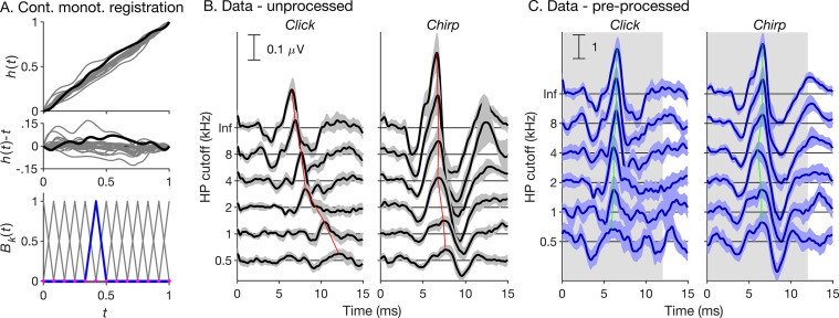
Fig. 2.

Continuous monotone registration approach [18] and test data. (A) Top and middle panels: Example time warping functions, h(t), constructed using the continuous monotone registration approach, and corresponding differences, h(t)−t, with the original time axis, t. Bottom panel: Linear B-spline functions (grey lines) used to model the logarithm of the first derivative of the warping functions, ln{h′(t)}. The thick blue line highlights one example B-spline. The purple dots represent the knots (see Section 3.3.1). (B) ABR data set used to test the proposed procedure. The left and right panels show different stimulus conditions (click and chirp). The horizontally staggered lines show different high-pass masking conditions (the ordinate shows the high-pass masker cutoff frequency in kHz; “Inf” signifies the broadband condition). The black lines show the average responses across subjects for each condition, and the grey-shaded areas show the corresponding cross-subject 95% confidence ranges. The thin red line connects the wave-V peak latencies across conditions. (C) Same data as in B, but after pre-processing (pre-alignment across high-pass masking conditions, cross-fading between 100- and 150-Hz high-pass-filtered versions, and normalization for root-mean-square amplitude; see Section 3.2.2). The grey highlight shows the warping time range (0–12 ms).