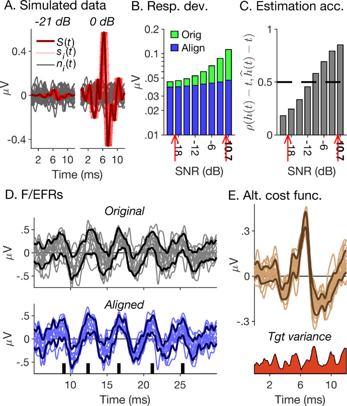
Fig. 7.

Simulated data and outlook. (A) Simulated ABRs. The dark red line shows the structural response, S(t), and the lighter red lines, the individual true ABRs, s(t). The grey lines show the individual noise traces. The left and right panels show the responses for the lowest and highest simulated SNRs (Δsnr = −21 and 0 dB), respectively. (B) Response deviations of the original (green bars) and aligned (blue bars) simulated responses as a function of their SNR (expressed as Δsnr for all conditions other than Δsnr = 0). The red arrows show the range of SNRs of the measured responses. (C) Estimation accuracy of time warping functions, measured as $\rho \left(h\left(t\right)-t,\widehat{h}\left(t\right)-t\right)$, as a function of SNR. (D&E) Possible future applications and extensions. (D) Non-linear curve registration could also be applied to frequency- or envelope-following responses (F/EFRs). This example shows responses to a short train of chirps, aligned using the at, PSDD, λ = 0 registration condition. The original and aligned responses are shown in the top and bottom panels, respectively. As in Fig. 5, the thinner, lighter-coloured lines show the individual responses and the thicker darker-coloured lines show their pointwise standard deviations. (E) In future, the criterion used for fitting the warping functions could take into account the variance as a function of time (bottom panel) of the target response (top panel; here, the aligned responses to the broadband chirp condition, replotted from Fig. 5A).