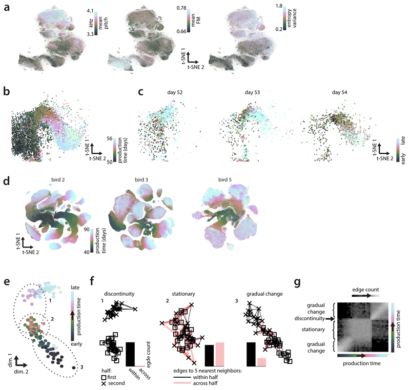
Extended Data Figure 2. Properties of large-scale embeddings.

(a) Three auditory features computed on renditions of syllable b. Same embedding as in Fig. 2a, but different coloring.

(b) Across-day change in vocalizations. Magnified cutout from Fig. 2a (bottom-left region of the dashed square). Coloring differs from Fig. 2a and only points from days 50-56 are shown.

(c) Within-day change in vocalizations. Points from (b) are shown separately for three individual days (top labels) and colored based on production time within the day (early to late; color bar). Vocalizations change within a day—early vocalizations (dark green) are more similar to vocalizations from previous days (dark green points in b); late vocalizations (light blue) are more similar to vocalization from future days (light blue in b).

(d) t-SNE visualizations for the continuous recordings of 3 birds (columns). Analogous to Fig. 2a.

(e-g) Illustration of a fictitious behavior undergoing distinct phases of abrupt change, no change, and gradual change, and the identification of these phases based on nearest neighbor graphs.

(e) A low-dimensional representation of the behavior. Each point corresponds to a behavioral rendition (e.g. a syllable rendition in the bird data) and is colored based on its production time. Similar renditions (e.g. that have similar spectrograms) appear near each other in this representation. The dotted ellipses mark three subsets of points corresponding to (1) a phase of abrupt change; (2) a phase of no change; and (3) a phase of gradual change.

(f) Nearest neighbor graphs for the three subsets of points in (e). Points are replotted from (e) with different symbols, indicating whether their production times fall within the first (squares) or second half (crosses) of the corresponding subset. Edges connect each point to its 5 nearest neighbors. Edge color marks neighboring pairs of points falling into the same (black) or different (red) halves. Relative counts of within- and across-half edges differ based on the nature of the underlying behavioral change (histograms of edge counts). If an abrupt change in behavior occurs between the first and second half, nearest neighbors of points in one half will all be points from the same half, and none from the other half (discontinuity). When behavior is stationary, the neighborhoods are maximally mixed, i.e. every point has about an equal number of neighbors from the two halves (stationary). Phases of gradual change result in intermediate levels of mixing (gradual change).

(g) Mixing-matrix for the simulated data in (e), analogous to Fig. 2e. Each location in the matrix corresponds to a pair of production times. Strong mixing (white) indicates a large number of nearest neighbor edges across the two corresponding production times (as in f, stationary) and thus similar behavior at the two times. Weak mixing (black) indicates a small number of such edges (as in f, discontinuity), and thus dissimilar behavior. Note that such statistics on the composition of local neighborhoods can be computed for any kind of behavior and are invariant with respect to transformations of the data that preserve nearest neighbors, like scaling, translation, or rotation. These properties make nearest neighbor approaches very general.