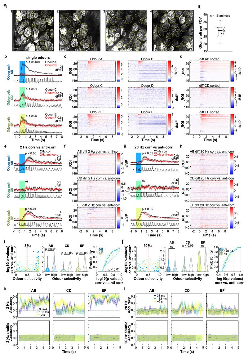
Extended Data Fig. 6. OSN imaging in response to correlated vs. anti-correlated odour stimulation.

a, Four example fields of view (FOV) recorded from the dorsal olfactory bulb of individual mice. aii, Number of individual glomeruli per FOV in all experimental mice (n = 15). The number of individually delineated glomeruli ranges from 20-36 with an average of 28 glomeruli per FOV. Labelled data points (1-4) correspond to FOVs shown in a_i. Scale bars: 50 μm. Edges of the box are the 25^th and 75^th percentiles, the whiskers extend to the most extreme data points not considered as outliers, see Methods. b, Example glomerulus response from OMP-Cre:Rosa-GCaMP6f mice to presentation of individual odours plotted pairwise (AB, CD, EF; mean of 6 trials ± SEM). Stimulation period (1 s) is indicated by vertical bar (blue, green and yellow). Bottom: Typical example respiration trace. P-values derived from unpaired two-sided t-tests comparing 2 s integrated responses between paired odours. c, Averaged calcium transients from all glomeruli (n = 145 from 5 individual animals) in response to individual odours, plotted as colour maps sorted by response magnitude. d, Difference between glomerulus responses to individual odours plotted pairwise as colour maps. Glomeruli are sorted by average magnitude of response difference. e, Example glomerulus response to presentation of correlated vs. anti-correlated odour pairs fluctuating at 2 Hz (mean of 12 trials ± SEM). Bottom: typical example respiration trace. P-values derived from unpaired two-sided t-tests comparing 2 s integrated responses of individual trials to correlated and anti-correlated odour stimulation. f, Difference between glomerulus responses to 2 Hz correlated and anti-correlated odours as colour maps sorted as shown in d. g-h, Same as in e-f but for 20 Hz correlated vs. anti-correlated. Example glomerulus from b,e,g indicated with an asterisk in colour maps in c,d,f,h. i, Left: P-values derived from comparing trials of the summed 2 s response to correlated vs. anti-correlated odour stimulation at 2 Hz (unpaired two-sided t-tests) for three odour pairs (colour-coded) as a function of glomerulus selectivity to individual odours (n = 145 glomeruli). Selectivity is calculated as the difference between the absolute response to single odours scaled by the summed absolute response. A threshold is set at 0.5 defining glomeruli as low or high selective. Dot size represents magnitude of the summed response. Middle: Comparison of p-values between low and high selective glomeruli (p < 0.05, unpaired two-sided t-test). Violin plots show the median as a white dot and the first and third quartile by the bounds of the grey bar. Right: Cumulative distribution function of p-values for low and high selective glomeruli (p < 0.01 for all pairwise comparisons, two-sample Kolmogorov-Smirnov test). j, Same as i but for 20 Hz, (n = 145 glomeruli). k, Top row: Mean ± SD over 100 repetitions of classifier accuracy when trained on all responsive glomeruli (n = 145 available, from 5 individual animals, see Methods) to discriminate 2 Hz correlated vs. anti-correlated stimuli, trained separately for each of the three odour pairs and within sliding windows of different widths (colours); x-coordinates indicate latest extent of each window. Bottom row: same as top row but with labels shuffled as control. l, Same as k for 20 Hz correlated vs. anti-correlated odours. Some data points in k, l are absent because not all time points had responsive ROIs for every window size (see Methods).