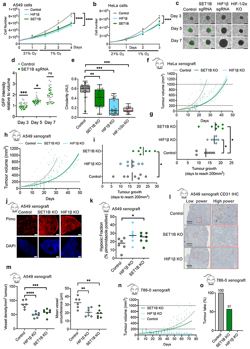
Fig. 4. Functional consequences of SET1B loss in hypoxia.
(a, b) Proliferation assays of HeLa (a) or A549 (b) depleted of HIF1B or SET1B grown in 21% or 1% oxygen for indicated number of days (n = 3 biologically independent samples, mean, P ≤ 0.0001, twoway ANOVA at 3 or 4 days). (c-e) HeLa control, SET1B-depleted, HIF-1β-depleted or HIF-1/2α clonal KO spheroids generated in HIF reporter cells. n = 54 (control), 39 (SET1B KO), 51 (HIF1β KO), 28 (HIF-1/2α KO) spheroids. Representative images (c) and GFP intensity (d) shown; control relative to SET1B depletion; P = 0.000003 day 3, P = 0.027 day 5,unpaired t-test. Scale bar 1.25 mm. (e) Circularity. Box and whisker plots show all points, min. to max., with 25th to 75th interquartile range box. Control vs. SET1B KO, P = 0.0037, control vs. HIF1β or HIF-1/2α KO P < 0.0001; Kruskal-Wallis for nonparametric data. (f-i) HeLa and A549 tumor xenograft models. (f, h) Tumor volumes measured (SET1B vs. control, P ≤ 0.0001, nonlinear regression F test). (g, i) Tumor establishment determined by time to reach 200 mm3 (n = 7 mice per condition, mean ± SD, P = 0.04 HeLa control vs. SET1B KO, P = 0.015 HeLa control vs. HIF1β KO, P = 0.048 A549 control vs. SET1B KO; unpaired two-tailed t-test). (j) Representative images of A549 tumor sections, harvested at > 1,000 mm3, stained with pimonidazole (red) and DAPI (blue). Scale bar 500 μm, n = 7 mice per condition. (k) Hypoxic tumor fraction in SET1B depletion vs. control, P = 0.035, unpaired t-test. n = 6 (control and HIF1β), 7 SET1B. (l) Representative IHC images of A549 tumor sections stained for blood vessels (CD31) (n = 7 mice per condition). (m) Vessel density (left) and mean vessel circumference (right) in A549 tumor sections. SET1B vs control density (P = 0.0009), and circumference (P = 0.001). HIF1β vs. control density (P ≤ 0.0001), and circumference (P = 0.003). n = 6 (control and HIF1β), 7 SET1B. mean ± SD, one-way ANOVA). (n, o) 786-0 tumor xenograft model. Tumor volume (SET1B vs. control, P ≤ 0.0001, nonlinear regression F test) (n) and the percentage of tumors that established (tumor take) are shown (o). Graphs show mean ± SD. * P < 0.05, ** P < 0.01, *** P < 0.001.

