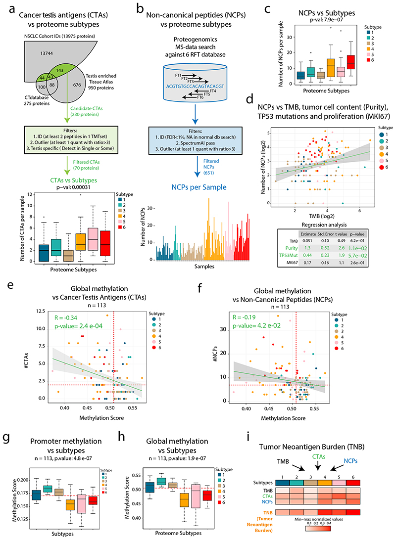
Figure 3. Cancer-Testis (CT) antigens, neoantigen burden and methylation in NSCLC.
a. Overview of cancer testis antigen (CTA) evaluation in NSCLC. Bottom part shows boxplot indicating the number of CTAs expressed per sample by proteome subtype (n = 141 samples). b. Overview of proteogenomic analysis by 6-reading frame translation (6FT) database searching. Lower part shows bar plot indicating the number of identified NCPs per sample (n = 141 samples). c. Boxplot indicating the number of non-canonical peptides (NCPs) per sample by proteome subtype (n = 141 samples). d. Scatter plot (top) showing the number of NCPs per sample vs TMB (n = 139 samples) and output from a multivariate linear regression analysis (bottom) between the number NCPs and TMB, tumor cell content (“purity”), TP53 mutations and proliferation (Ki67 quantified by MS) (n = 139 samples). e-f. Scatter plot indicating the global methylation plotted against the number of CT antigens per sample or the number of NCPs per sample (n = 113 samples). g-h. Boxplots indicating the global and promoter methylation by proteome subtype (n = 113 samples). i. Heatmap showing Tumor Neoantigen Burden (TNB) by proteome subtype where TNB is defined as a summary score based on TMB, CTAs and NCPs. In figures e, f, g, and h, red dotted lines indicate median values and the number of samples with quantitative information at both methylation and protein level is provided. For scatter plots d, e, and f: Samples are colored by proteome subtype. The number of samples with quantitative information at both methylation and protein level is provided and a linear regression trendline is displayed in green. 95% confidence intervals are shown in grey. The associated Pearson’s correlation coefficients (Rho) and two-sided p-values from t-distribution with n − 2 degrees of freedom are provided. For boxplots a, c, g, and h: middle line, median; box edges, 25th and 75th percentiles; whiskers, most extreme points that do not exceed ±1.5 × the interquartile range (IQR). P-values were calculated by Kruskal-Wallis test. Dunn’s multiple comparison tests with Benjamini-Hochberg adjustment for boxplots are available in Supplementary Table 3.

