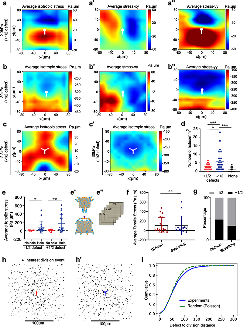
Extended Data Fig. 5. Defect mediated tensile stress and its association with hole formation.

(a, b) Averaged isotropic stress, averaged stress xy (a’, b’) and averaged stress yy (a”, b”) around +1/2 defects on soft (2.3kPa) gels (a, a’, a”) (n = 2924 defects) and stiff (30kPa) gels (b, b’, b”) (n = 3632 defects) from 2 independent experiments. (c, c’) Averaged isotropic stress around -1/2 defects on (c) soft (2.3kPa) gel (n = 2810 defects) and (c’) stiff (30kPa) gels (n = 3716 defects) from 2 independent experiments. White dots indicate the location of the defect core. (d) Number of holes per mm² that are triggered by each defect type in the preceding frame in comparison to regions where defects do not lead to hole formation (n=20 circles from 4 independent experiments; *p < 0.01, ***p < 0.001). Error bars represent standard deviation. (e) Averaged peak isotropic stress around a region of 25.6x25.6μm obtained from a random defect that does not lead to a hole site and defects that lead to hole formation (n_{-1/2 random no-hole and hole}=16, n_{+1/2 random and hole}=17; *p < 0.01, **p < 0.05) from 3 independent experiments. While a region around the defect centre was averaged for -1/2 defects, for +1/2 defects stresses were averaged in the tail region of the defect. Error bars represent standard deviation. As shown in (e’) a region around the defect centre was averaged for -1/2 defects, for +1/2 defects stresses were averaged in the tail region of the defect. Peak areal averaged stress within a time frame of 20-40 minutes prior to hole formation was obtained as shown in (e”). Error bars represent standard deviation. (f) Average tensile stress around defect that leads to cell division or stretching related hole formation (n_{cell_div} = 19, n_stretching = 13) (g) Percentage of +/- 1/2 linked division and stretched cell linked hole formation on 2.3kPa gels from 4 independent experiments. Error bars represent standard deviation. (h-h’) Scatter plot in the location of the nearest cell division (with the cell separation detected in the next frame) to (h) a +1/2 defect and (h’) a +1/2 defect. The spatial pattern displays no bias towards a particular region of space, as in the case of a random distribution of points. (i) cumulative distribution, which highlights the difference between the two distributions; relatively minor differences arise at large distances (100-150 microns).