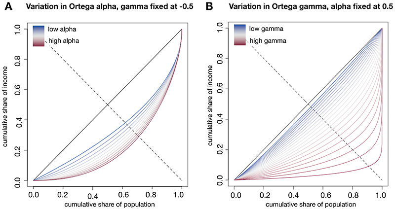
Fig. 3. Using simulations to systematically vary the two Ortega parameters to identify their impact on the shape of the income distribution.
A. The disproportionate change exhibited by the Lorenz curve varying the Ortega parameter α within the range of 0.01 to 1.5 leads to a more pronounced change for lower income percentiles. (The dotted off-diagonal line facilitates the recognition that the Lorenz curve is stretched more intensely in lower income percentiles.) B. Conversely, varying the Ortega parameter γ within the range 0.01 to 0.99, the Lorenz curve exhibits a disproportionate change in the top income percentiles. For comparison, the empirical estimates across counties for α range from 0.12 to 1.23 and for γ range from 0.3 to 0.93.

