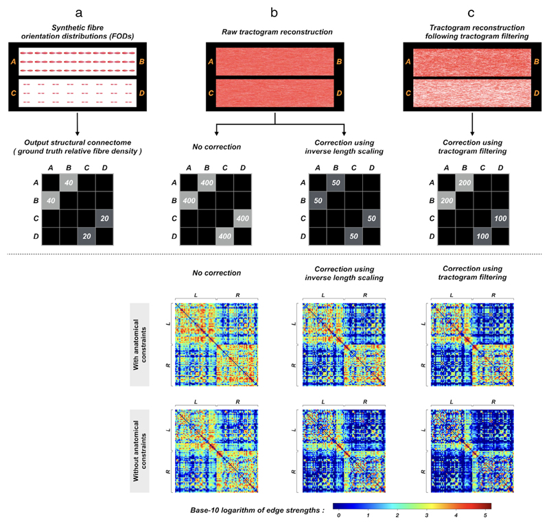
Figure 4.

The effects of quantitative tractogram postprocessing on subsequent quantification of connectome construction, illustrated using a synthetic example (upper panel) and human image data (bottom panel): Upper panel: (a) Fiber bundles A$B and C$D are simulated using synthetic fiber orientation distributions (FODs), where the size of FODs (i.e., apparent fiber density⁵⁸) in A$B is twice that in C$D. The relative fiber density of this synthetic FOD field is reflected in the connectome. (b) When running fiber-tracking, no matter whether seeding is performed uniformly from the whole (i.e., mimicking WM seeding) or from the extremities (i.e., mimicking seeding at the interface between GM and WM) of the fiber bundles, the same number of streamlines will be generated in both pathways. Obviously, the results do not comply with the synthetic ground-truth. The resultant connectome edges weighted by streamline density are therefore also biased in A$B and C$D when no correction is applied. Also, as inverse length scaling does not consider the size of FODs, it cannot correct for this type of quantification bias. (c) With the application of quantitative tractogram processing techniques (e.g., using Refs. 42, 45), the reconstructed streamline densities are rendered consistent with the underlying FOD field in A$B and C$D, making the connectome edges weighted by streamline density linearly proportional to the actual fiber density.

Bottom panel: Group-averaged connectivity matrices generated from a cohort of healthy subjects. Probabilistic tractograms are generated with WM seeding; nodes are defined by the Desikan–Killiany atlas⁴⁸; edges are defined by streamline count. The first row shows the connectomes obtained from tractograms with anatomical constraints and then processed by different levels of quantitative bias correction (left: no correction; middle: correction using inverse length scaling; right: correction using tractogram filtering). For comparisons, the bottom row shows the results without anatomically-constrained tracking. L and R denote left and right hemispheres, respectively. The differences among these connectivity matrices are clearly visible, and indeed a range of popular connectomic metrics are significantly different.⁴³ This figure is adapted from Ref. 43 with copyright permission.