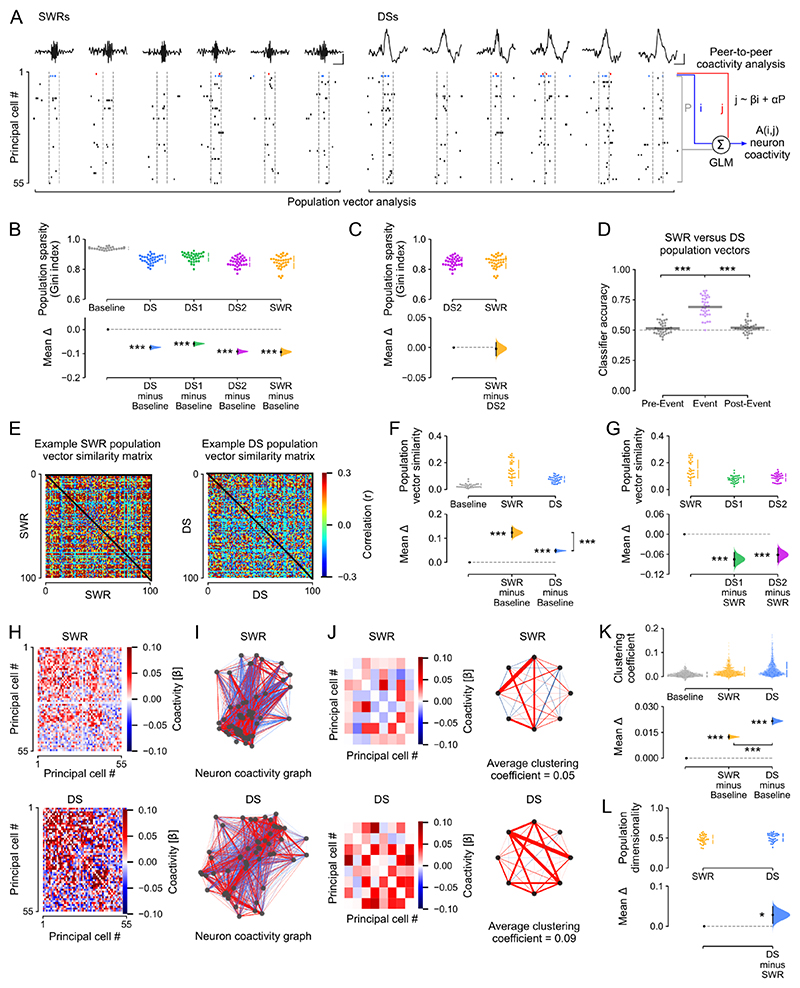
Figure 3. The coactivity structure of population spiking differs between DSs and SWRs.

(A) Analytical framework: the population-level coactivity structure was analyzed using population vectors of principal cell spiking transiently nested in individual SWRs, DSs, or duration-matched (50 ms) baseline control windows. Scale bars show 20ms and 0.5mV for SWRs and 1mv for DSs. For the analyses in panels B-G, these population firing vectors were then binarized (for each cell: a non-zero spike count gives 1; or else 0). For the analyses in H-K, we calculated the peer-to-peer coactivity, controlling for the overall population activity.

(B, C) Estimation plots showing the effect size for the differences in population sparsity (using the Gini index) during DSs (with DS₁ and DS₂ plotted altogether or separately), SWRs, and compared to equivalent (50 ms duration matched) baseline windows (Baseline) in which no DSs or SWRs occurred. Upper: raw data points (each point represents one session with at least 100 of each event type and 20 principal cells), with the gapped lines on the right as mean (gap) ± s.d. (vertical ends) for each event. Lower: difference (Δ) in sparsity between Baseline windows and all DS, DS₁, DS₂, and SWR events computed from 5,000 bootstrapped resamples and with the difference-axis origin (dashed line) aligned to the baseline sparsity (black dot, mean; black ticks, 95% confidence interval; filled curve, sampling-error distribution). (C) as B but comparing population sparsity during SWR versus DS₂. Note that DS₂ and SWR events have equivalent sparsity, indicating they engage similar levels of neuronal activity.

(D) A logistic regression classifier trained on population vectors nested in SWR versus DS events, or matched duration pre-event and post-event control windows, using a 4-fold cross-validation approach (75% of vectors for training; the remaining 25% for evaluation), significantly discriminated DSs from SWRs, but could not discriminate between pre-DS versus pre-SWR, and post-DS versus post-SWR vectors. Gray horizontal bars: mean classification accuracy.

(E-G) DS population firing vectors are more diverse than those in SWRs. For each sleep session, we computed the similarity (Pearson correlation coefficient) for each pair of population vectors nested in either DSs, SWRs, or duration-matched baseline windows (Baseline). (E) shows example DS and SWR matrices of cross-vector similarity for one session. Cross-population vector similarity was significantly higher in SWRs compared to both DSs and control windows (F), and when compared to DS₁ and DS₂ separately (G).

(H-K) DS and SWR population firing vectors exhibit distinct topology of neuronal coactivity. The coactivity between any two (i, j) neurons was measured using a GLM that quantified their short timescale (50 ms windows centered on DS or SWR peaks) firing relationship while accounting for network-level modulation reported by the remaining principal cells in the population (A). (H) This procedure returned for both DS and SWR events an adjacency matrix of β regression weights that represented the neuron pairwise coactivity structure of the population (example matrix from one session). (I) Visualization of the corresponding matrices representing DS and SWR based neuronal coactivity graphs. For clarity, (J) shows an example subset (left) for each adjacency matrices shown in (H), along with its corresponding motifs of neuronal coactivity and average clustering coefficient (right). (K) Note that DS-based graphs contained stronger triads of coactive nodes compared to both SWR graphs and control graphs constructed from duration-matched baseline windows (Baseline), as indicated by higher mean clustering coefficients. Each point in the upper plot of K represents the mean clustering coefficient for one hippocampal principal cell (n=1265 neurons, 8 mice)

(L) The dimensionality of population vector matrices (number of principal components required to explain 90% of the variance) was higher for DSs than SWRs.

For B-D, F-G, L: each data point shows one recording session (n=34 recording sessions from 8 mice). The test statistic is the mean difference, shown on the y-axis of each lower plot. P-values are from paired permutation tests, event versus baseline (B,F,K); event versus event (C,F,K,L); or event versus pre-event, event versus post-event (D), *P < 0.05, **P < 0.01, ***P < 0.001.