Control of COVID-19 system using a novel nonlinear robust control algorithm

Highlights

• •A new topic (COVID-19 epidemic) has been introduced in the literature of control theory. In addition, a new robust control algorithm has been applied to the COVID-19 nonlinear system after making some assumptions.
• •The data of the paper are valid for a certain period of time and the controller could be applied to the same system with different data.
• •The stability of the system has been achieved using Lyapunov stability analysis and the system performance has been improved much better. Moreover, the parameters of the proposed controller have been optimized using new optimization method called the Most Valuable Player Algorithm (MVPA). The MVPA has introduced for the first time to the literature of control theory.

Abstract

COVID-19 has been a worldwide concern since the outbreak. Many strategies have been involved such as suppression and mitigation strategies to deal with this epidemic. In this paper, a new mathematical-engineering strategy is introduced in order to control the COVID-19 epidemic. Thereby, control theory is involved in controlling the unstable epidemic alongside with the other suggested strategies until the vaccine will hopefully be invented as soon as possible. A new robust control algorithm is introduced to compensate the COVID-19 nonlinear system by propose a proper controller after using necessary assumptions and analysis are made. In addition, the Variable Transformation Technique (VTT) is used to simplify the COVID-19 system. Furthermore, the Most Valuable Player Algorithm (MVPA) is applied in order to optimize the parameters of the proposed controller. The simulation results are based on the daily reports of two cities Hubei (China) and Lazio (Italy) since the outbreak. It can be concluded that the proposed control algorithm can effectively compensate the COVID-19 system. In addition, it can be considered as an effective mathematical-engineering strategy to control this epidemic alongside with the other strategies.

1. Introduction

In the late of December 2019, a group of pneumonia cases was identified in Wuhan (China). It was discovered that these cases were caused by β-coronavirus or what yet initially named as the 2019-novel Coronavirus (2019-nCoV) on 12 January 2020 by World Health Organization [1]. Later, WHO officially named the disease as Coronavirus disease 2019 (COVID-19), while Coronavirus Study Group (CSG) suggested to name this virus as SARS-CoV-2, both issued on 11 February 2020. After that, the number of the cases were rapidly increased in Wuhan. Consequently, The Chinese scientists decided to isolate a SARS-CoV-2 from a patient within a short time on 7 January 2020 and came out to genome sequencing of the SARS-CoV-2 [2,3]. In 1 March 2020, a total number of reported cases were 79,968 including 2873 deaths of the COVID-19 were confirmed in China (Coronavirus disease 2020). Studies estimated the basic reproduction number ($R_0$) of COVID-19 to be around 2.2 or even more (1.4–6.5) and familial clusters of pneumonia outbreaks add to evidence of the epidemic SARS-CoV-2 constantly increasing by human-to-human transmission [[4], [5], [6]].

There are two recommended strategies to handle the COVID-19 outbreak suppression and mitigation. First, suppression which is an approach of apply a strict social distancing policies that have been taken by governments such as applying stay-at-home orders, shut down public places, commercial activities, non-essential industrial activities and schools, stopping all kinds of travels, …, etc. The aim of this strategy is to decrease the number of the reproduction $R_t$, which represents the number of the infectious persons; this was applied in China. This approach was followed very thoroughly by China effectively for couple of months [7,8]. Second, mitigation which is a strategy that means letting the COVID-19 epidemic complete its course in a controlled way such as the idea of herd immunity. This strategy was initially applied by UK government, which becomes ineffective therefore, it was replaced with suppression strategy after the public release of report [9,10].

The contribution of this paper is to involve the fundamental of the control theory to provide a control engineering insight strategy in order to reduce the COVID-19 epidemic. Consequently, SEIR model is developed to represents the dynamical COVID-19 nonlinear system after some assumptions are made. Furthermore, a robust control algorithm is applied to compensate the nonlinearity, instability of the COVID-19 nonlinear system. Eventually, the results of the model were based on the daily reports in both Hubei (China) and Lazio at the beginning of the COVID-19 outbreak.

The rest of the paper is organized as follows. The robust control algorithm is introduced in Section 3 with COVID-19 mathematical description, Variable Transformation Technique (VTT) and Most Valuable Player Algorithm (MVPA). The simulation results are explained in Section 4 in order to show the potential effects of the control algorithm. In Section 5, the discussion is made to sum up the results and discuss the final evaluation of the proposed control algorithm. Eventually, the conclusion is presented in Section 6.

2. Materials and methods

In this section, a new robust control algorithm is introduced in order to compensate the COVID-19 nonlinear system. In addition, the mathematical model of the COVID-19 is presented with a necessary assumptions and new techniques/methods that are used alongside with the proposed control algorithm to fit the design procedure.

2.1. Covid-19 mathematical model description

The basic Susceptible-Exposed-Infectious-Recovered (SEIR) model can be developed as COVID-19 model as follows [11]:

$$\frac{\mathit{d}\mathit{S}(\mathit{t})}{\mathit{d}\mathit{t}}=-\frac{\mathit{\beta }\mathit{I}(\mathit{t})\mathit{S}\left(\mathit{t}\right)}{\mathit{N}}$$ (1)

$$\frac{\mathit{d}\mathit{E}(\mathit{t})}{\mathit{d}\mathit{t}}=\frac{\mathit{\beta }\mathit{I}\left(\mathit{t}\right)\mathit{S}(\mathit{t})}{\mathit{N}}-\mathit{\epsilon }\mathit{E}(\mathit{t})$$ (2)

$$\frac{\mathit{d}\mathit{I}(\mathit{t})}{\mathit{d}\mathit{t}}=\mathit{\epsilon }\mathit{E}(\mathit{t})-\mathit{\gamma }\mathit{I}(\mathit{t})$$ (3)

$$\frac{\mathit{d}\mathit{R}(\mathit{t})}{\mathit{d}\mathit{t}}=\mathit{\gamma }\mathit{I}(\mathit{t})$$ (4)

where $R(t)$ represents Resistant subjects, $S(t)$ represents Susceptible individuals, $I(t)$ represents Infectious individuals that have infected but are not yet infectious, $N$ represents the total population and $E(t)$ represents Exposed individuals. The parameter $\beta$ represents the likelihood of infection per unit time; $\epsilon$ refers to the inverse of the average latency time of the disease, and $\gamma$ represents the inverse of the average time infectious individuals spend by actually infecting other people.

The following are assumptions of the COVID-19 outbreak in Europe which are helps to reduce the abovementioned system (Eqs. (1), (2), (3), (4)) to a second order control system [12]:

• 1)Given low mortality percentage, births and deaths are neglected and the short time spans involved.
• 2)Emigration and immigration are also ignored for simplicity.
• 3)Adding Eqs. (1), (2), (3), (4) gives:

$$\frac{\mathit{d}(\mathit{S}(\mathit{t})+\mathit{E}(\mathit{t})+\mathit{I}(\mathit{t})+\mathit{R}(\mathit{t}))}{\mathit{d}\mathit{t}}=0$$ (5)

$$\text{T}\text{h}\text{e}\text{r}\text{e}\text{f}\text{o}\text{r}\text{e},\mathit{R}\left(\mathit{t}\right)=\mathit{N}-\mathit{S}(\mathit{t})+\mathit{E}(\mathit{t})+\mathit{I}(\mathit{t})$$ (6)

• 4)COVID-19 (or SARS-CoV-2) virus is a new virus therefore, the vast majority of the people around the world have never been exposed to it yet.
• 5)There is no effective vaccine or cure for the virus.
• 6)The positive tested ratio depends mainly on the country and it is ranging from about $2\%$ like Germany to about $10\%$ like Italy, France and Spain.
• 7)The real mortality ratio corresponding to infected people is very low, since many cases have shown no issues and these are not tested positive for the COVID-19 virus but they are still infectious. The ratio between positive tested cases and really infectious cases is called $\alpha$ ratio which is around one order of magnitude, mainly country dependent and uncertain. In the case of the Hubei province outbreak it was estimated that $\alpha =0.05$ [10].
• 8)A particular fraction of official reports of the infectious subjects ends up developing severe bilateral respiratory difficulties and pneumonia difficulties which need hospitalization. A smaller fraction $\sigma$ of cases around $4\%$ in Northern Italy eventually requires very intensive care to keep the patient’s life functions, mechanical ventilation or he is likely to die if this is not available.
• 9)The number of beds in public health systems is normally needs based such as rare disease care, post-surgery care and trauma care. Moreover, the additional of COVID-19 patients $N_{ic}$ that can be admitted to intensive care is thus severely limited of the order of ${10}^{-4}N$ in developed countries. This number of the patients can be expanded significantly if action is taken in time but certainly not by orders of magnitude.
• 10)The initial action of the outbreak dynamics is so fast, with times of reported cases that is doubled of the order of $4$ days.
• 11)In many cases, people are tested only after they are shown serious symptoms of the virus, which made on average ${\tau }_t$ days after they were being infectious.
• 12)The testing procedure also presents a time delay ${\tau }_r$ in the process. Although it is possible to come out the results of the test in a few hours. However, the time average of the reports is longer because of the limitation in the equipments, for example about $1$ week in Italy.

To sum up some assumptions, Item 4 proposes to consider $S(0)=N$. The absence of a vaccine (Item 2) includes there is no means to decrease the value of $S$ and grow the value of $R$ by means of vaccination campaigns. Item 6 permit us to consider $\gamma$ and $\epsilon$ as constants. Items 7,8 are combined to Items 4–6 which are critical from the modeling prospective.

Moreover, in the first three months of the COVID-19 outbreak the number $R$ of publication who recover are small compared to the overall population. Therefore, $E(t)+I\left(t\right)+R(t)<<S(t)$ but $R(t)+E(t)+I(t)+S(t)=N$, it can be assumed in Eqs. (2), (3) that $S$ is constant, and almost equals to $N$. By decoupling Eqs. (2), (3) from Eq. (1) gives [12]:

$$\frac{\mathit{d}\mathit{E}(\mathit{t})}{\mathit{d}\mathit{t}}=\mathit{\beta }\mathit{I}(\mathit{t})-\mathit{\epsilon }\mathit{E}(\mathit{t})$$ (7)

$$\frac{\mathit{d}\mathit{I}(\mathit{t})}{\mathit{d}\mathit{t}}=\mathit{\epsilon }\mathit{E}(\mathit{t})-\mathit{\gamma }\mathit{I}(\mathit{t})$$ (8)

However, the $\sigma$ empirical ratio of patients need an intensive care as in Item 8 is pointed out to the lower number $I_t(t)=\alpha I(t)$ of people who are finally tested positive to the virus. Assuming $\alpha$ considered as a constant, Eqs. (7), (8) are hold for $I_t(t)$ and $E_t(t)$. The interventions of the government previously mentioned decrease the $\beta$ which is the rate of infection, hence the real number of the reproduction $R_t=\gamma =\beta$. In fact, it can be assumed that the time-varying parameter β is functional (a function of another function $u(t)$) with $u$ indicating that may contain the cure part in the future. Therefore, the control-oriented model of epidemic is thus [12]:

$$\frac{\mathit{d}{\mathit{E}}_{\mathit{t}}(\mathit{t})}{\mathit{d}\mathit{t}}=\mathit{\beta }(\mathit{u}\left(\mathit{t}\right)){\mathit{I}}_{\mathit{t}}(\mathit{t})-\mathit{\epsilon }{\mathit{E}}_{\mathit{t}}(\mathit{t})$$ (9)

$$\frac{\mathit{d}{\mathit{I}}_{\mathit{t}}(\mathit{t})}{\mathit{d}\mathit{t}}=\mathit{\epsilon }{\mathit{E}}_{\mathit{t}}\left(\mathit{t}\right)-\mathit{\gamma }{\mathit{I}}_{\mathit{t}}(\mathit{t})$$ (10)

$$\mathit{y}\left(\mathit{t}\right)=\mathit{\epsilon }{\mathit{E}}_{\mathit{t}}\left(\mathit{t}\right)$$ (11)

In the next section, the Variable Transformation Technique (VTT) is used to reformulate the COVID-19 system in order to fit the analysis procedure of the proposed control algorithm.

2.2. Variable transformation technique

In this subsection, the Variable Transformation Technique (VTT) is introduced to overcome the complexity of the structures in the nonlinear systems such as COVID-19. It can be derived by using the recursive derivative of the first state in order to find other states to be transformed based on pre-assumptions. VTT uses basic Calculus to deal with complex structures in order to be transformed to the proper form [13]. The following is the Variable Transformation Technique (VTT) procedure which is used to simplify the complicated structures instead of using cumbersome and complex design steps in the traditional backstepping technique:

$$\text{S}\text{t}\text{e}\text{p}1:\text{L}\text{e}\text{t}{\mathit{z}}_1={\mathit{x}}_1,{\dot{\mathit{z}}}_1={\dot{\mathit{x}}}_1$$ (12)

$$\text{S}\text{t}\text{e}\text{p}2:\text{L}\text{e}\text{t}{\mathit{z}}_2={\dot{\mathit{z}}}_1={\mathit{f}}_1({\mathit{x}}_1,{\mathit{x}}_2)$$ (13)

$${\dot{\mathit{z}}}_2={\ddot{\mathit{x}}}_1=\frac{\partial {\mathit{f}}_1({\mathit{x}}_1,{\mathit{x}}_2)}{\partial {\mathit{x}}_1}{\dot{\mathit{x}}}_1+\frac{\partial {\mathit{f}}_2({\mathit{x}}_1,{\mathit{x}}_2)}{\partial {\mathit{x}}_2}{\dot{\mathit{x}}}_2={\ddot{\mathit{x}}}_1=\frac{\partial {\mathit{f}}_1\left({\mathit{x}}_1,{\mathit{x}}_2\right)}{\partial {\mathit{x}}_1}{\mathit{f}}_1\left({\mathit{x}}_1,{\mathit{x}}_2\right)+\frac{\partial {\mathit{f}}_2\left({\mathit{x}}_1,{\mathit{x}}_2\right)}{\partial {\mathit{x}}_2}{\mathit{f}}_2\left({\mathit{x}}_2,{\mathit{x}}_3\right)={\mathit{F}}_1({\mathit{x}}_3)$$ (14)

The next steps can be written as follow:

$$\begin{array}{c}{\dot{\mathit{z}}}_{\mathit{i}}={\mathit{x}}_1^{(\mathit{i})}={\dot{\mathit{z}}}_{\mathit{i}-1}\\ =\frac{\partial {\mathit{F}}_{\mathit{i}-2}({\mathit{x}}_{\mathit{i}})}{\partial {\mathit{x}}_1}{\dot{\mathit{x}}}_1+\frac{\partial {\mathit{F}}_{\mathit{i}-2}({\mathit{x}}_{\mathit{i}})}{\partial {\mathit{x}}_1}{\dot{\mathit{x}}}_2+\cdots +\frac{\partial {\mathit{F}}_{\mathit{i}-2}\left({\mathit{x}}_{\mathit{i}}\right)}{\partial {\mathit{x}}_{\mathit{i}}}{\dot{\mathit{x}}}_{\mathit{i}},(3\le \mathit{i}\le \mathit{n}-1)\\ =\frac{\partial {\mathit{F}}_{\mathit{i}-2}({\mathit{x}}_{\mathit{i}})}{\partial {\mathit{x}}_1}{\mathit{f}}_1\left({\mathit{x}}_2\right)+\frac{\partial {\mathit{F}}_{\mathit{i}-2}({\mathit{x}}_{\mathit{i}})}{\partial {\mathit{x}}_2}{\mathit{f}}_2\left({\mathit{x}}_3\right)+\cdots +\frac{\partial {\mathit{F}}_{\mathit{i}-2}\left({\mathit{x}}_{\mathit{i}}\right)}{\partial {\mathit{x}}_{\mathit{i}}}{\mathit{f}}_{\mathit{i}}\left({\mathit{x}}_{\mathit{i}+1}\right)\end{array}$$ (15)

$$={\mathit{F}}_{\mathit{i}-1}({\mathit{x}}_{\mathit{i}+1})$$ (16)

where ${\mathit{F}}_{\mathit{i}-2}({\mathit{x}}_{\mathit{i}})$ can be found from Eq. (16).

The process is repeated to the number of the states $n$

$$\begin{array}{c}\text{S}\text{t}\text{e}\text{p}n:\text{L}\text{e}\text{t}{\dot{\mathit{z}}}_{\mathit{n}}={\mathit{x}}_1^{(\mathit{n})}={\dot{\mathit{z}}}_{\mathit{n}-1}\\ =\frac{\partial {\mathit{F}}_{\mathit{n}-2}({\mathit{x}}_{\mathit{n}})}{\partial {\mathit{x}}_1}{\dot{\mathit{x}}}_1+\frac{\partial {\mathit{F}}_{\mathit{n}-2}({\mathit{x}}_{\mathit{n}})}{\partial {\mathit{x}}_1}{\dot{\mathit{x}}}_2+\cdots +\frac{\partial {\mathit{F}}_{\mathit{n}-2}\left({\mathit{x}}_{\mathit{n}}\right)}{\partial {\mathit{x}}_{\mathit{n}}}{\dot{\mathit{x}}}_{\mathit{n}}\\ =\frac{\partial {\mathit{F}}_{\mathit{n}-2}({\mathit{x}}_{\mathit{n}})}{\partial {\mathit{x}}_1}{\mathit{f}}_1\left({\mathit{x}}_2\right)+\frac{\partial {\mathit{F}}_{\mathit{n}-2}({\mathit{x}}_{\mathit{n}})}{\partial {\mathit{x}}_2}{\mathit{f}}_2\left({\mathit{x}}_3\right)+\cdots +\frac{\partial {\mathit{F}}_{\mathit{n}-2}\left({\mathit{x}}_{\mathit{n}}\right)}{\partial {\mathit{x}}_{\mathit{i}}}{\mathit{f}}_{\mathit{n}}\left({\mathit{x}}_{\mathit{n}},\mathit{u}\right)\end{array}$$ (17)

$$={\mathit{F}}_{\mathit{n}-1}({\mathit{x}}_{\mathit{n}},\mathit{u})$$ (18)

where ${\mathit{F}}_{\mathit{n}-2}({\mathit{x}}_{\mathit{n}})$ can be found from Eq. (18).

Finally, the new system which is equivalent to the actual system is presented as follow:

$$\begin{array}{c}{\dot{\mathit{z}}}_1={\mathit{z}}_2\\ {\dot{\mathit{z}}}_2={\mathit{z}}_3\\ \begin{array}{c}⋮\\ {\dot{\mathit{z}}}_{\mathit{n}}={\mathit{F}}_{\mathit{n}-1}({\mathit{x}}_{\mathit{n}},\mathit{u})\end{array}\end{array}$$ (19)

It’s obvious that the system in (19) is simpler than many actual systems which have complex structures. Consequently, the output of the actual system equals to a state or number of states summed together which can be transformed in the same abovementioned technique.

2.3. Robust control algorithm

First of all, the VTT is applied in order to simplify the COVID-19 system as follow:

$$\text{L}\text{e}\text{t}{\mathit{z}}_1={\mathit{I}}_{\mathit{t}}\left(\mathit{t}\right),{\dot{\mathit{z}}}_1=\frac{\mathit{d}{\mathit{I}}_{\mathit{t}}(\mathit{t})}{\mathit{d}\mathit{t}}=\mathit{\epsilon }{\mathit{E}}_{\mathit{t}}\left(\mathit{t}\right)-\mathit{\gamma }{\mathit{I}}_{\mathit{t}}\left(\mathit{t}\right)={\mathit{z}}_2$$ (20)

$$\text{T}\text{h}\text{e}\text{n}{\mathit{E}}_{\mathit{t}}\left(\mathit{t}\right)=\frac{{\mathit{z}}_2-\mathit{\gamma }{\mathit{z}}_1}{\mathit{\epsilon }}$$ (21)

$$\text{T}\text{h}\text{e}\text{r}\text{e}\text{b}\text{y}{\dot{\mathit{z}}}_2={\ddot{\mathit{z}}}_1=\mathit{\epsilon }{\dot{\mathit{E}}}_{\mathit{t}}\left(\mathit{t}\right)-\mathit{\gamma }{\dot{\mathit{I}}}_{\mathit{t}}\left(\mathit{t}\right)=\mathit{\epsilon }(\mathit{\beta }(\mathit{u}\left(\mathit{t}\right)){\mathit{I}}_{\mathit{t}}(\mathit{t})-\mathit{\epsilon }{\mathit{E}}_{\mathit{t}}(\mathit{t}))-\mathit{\gamma }{\dot{\mathit{I}}}_{\mathit{t}}\left(\mathit{t}\right)=\mathit{\epsilon }\mathit{\beta }(\mathit{u}\left(\mathit{t}\right)){\mathit{I}}_{\mathit{t}}(\mathit{t})-{\mathit{\epsilon }}^2{\mathit{E}}_{\mathit{t}}(\mathit{t})-\mathit{\gamma }{\dot{\mathit{I}}}_{\mathit{t}}\left(\mathit{t}\right)$$ (22)

Substituting Eqs. (20) and (21) in Eq. (22) gives:

$$=\mathit{\epsilon }\mathit{\beta }(\mathit{u}\left(\mathit{t}\right)){\mathit{z}}_1-{\mathit{\epsilon }}^2(\frac{{\mathit{z}}_2-\mathit{\gamma }{\mathit{z}}_1}{\mathit{\epsilon }})-\mathit{\gamma }{\mathit{z}}_2$$

$$=\mathit{\epsilon }\mathit{\beta }\left(\mathit{u}\left(\mathit{t}\right)\right){\mathit{z}}_1-\mathit{\epsilon }{\mathit{z}}_2+\mathit{\epsilon }\mathit{\gamma }{\mathit{z}}_1-\mathit{\gamma }{\mathit{z}}_2$$

$$=\mathit{\epsilon }\mathit{\gamma }{\mathit{z}}_1-\left(\mathit{\epsilon }+\mathit{\gamma }\right){\mathit{z}}_2+\mathit{\epsilon }\mathit{\beta }\left(\mathit{u}\left(\mathit{t}\right)\right){\mathit{z}}_1$$

The new system becomes as follow:

$$\begin{array}{c}\left[\begin{array}{c}\dot{{\mathit{z}}_1}\\ \dot{{\mathit{z}}_2}\end{array}\right]=\left[\begin{array}{cc}0& 1\\ \mathit{\epsilon }\mathit{\gamma }& -\left(\mathit{\epsilon }+\mathit{\gamma }\right)\end{array}\right]\left[\begin{array}{c}{\mathit{z}}_1\\ {\mathit{z}}_2\end{array}\right]+\left[\begin{array}{c}0\\ {\mathit{\epsilon }\mathit{z}}_1\end{array}\right]\mathit{\beta }\left(\mathit{u}\left(\mathit{t}\right)\right)\\ \dot{\mathit{z}}=\mathit{f}\left(\mathit{z},\mathit{u},\mathit{t}\right)\end{array}$$ (23)

Now, the Lyapunov Quadratic Function (LQF) is used to analyze the system and figure out a proper controller to stabilize and control the COVID-19 epidemic. Since, the number of states in the actual systems is$n=2$, then, a second order model reference is selected to fit the design procedure as follows [14]:

$${\dot{\mathit{z}}}_{\mathit{d}}=\mathit{A}{\mathit{z}}_{\mathit{d}}+\mathit{B}\mathit{r}$$ (24)

$$\left[\begin{array}{c}{\dot{\mathit{z}}}_1\\ {\dot{\mathit{z}}}_2\end{array}\right]=\left[\begin{array}{cc}0& 1\\ -\mathit{a}& -\mathit{b}\end{array}\right]\left[\begin{array}{c}{\mathit{z}}_1\\ {\mathit{z}}_2\end{array}\right]+\left[\begin{array}{c}0\\ \mathit{a}\end{array}\right]\mathit{r}$$ (25)

where $a$, $b$ are positive constants and $r$ is step input.

The error between the model reference and the actual system can be defined as follow:

$$\begin{array}{c}\mathit{e}={\mathit{z}}_{\mathit{d}}-\mathit{z}\\ \dot{\mathit{e}}={\dot{\mathit{z}}}_{\mathit{d}}-\dot{\mathit{z}}\end{array}$$ (26)

Substituting Eq. (23) and Eq. (24) in Eq. (26) gives:

$$\begin{array}{c}\dot{\mathit{e}}=\mathit{A}{\mathit{z}}_{\mathit{d}}+\mathit{B}\mathit{r}-\mathit{f}\left(\mathit{z},\mathit{u},\mathit{t}\right)\\ \dot{\mathit{e}}=\mathit{A}{\mathit{z}}_{\mathit{d}}+\mathit{B}\mathit{r}-\mathit{f}\left(\mathit{z},\mathit{u},\mathit{t}\right)+\mathit{A}\mathit{z}-\mathit{A}\mathit{z}\\ \begin{array}{c}\dot{\mathit{e}}=\mathit{A}\left({\mathit{z}}_{\mathit{d}}-\mathit{z}\right)+\mathit{A}\mathit{z}+\mathit{B}\mathit{r}-\mathit{f}\left(\mathit{z},\mathit{u},\mathit{t}\right)\\ \dot{\mathit{e}}=\mathit{A}\mathit{e}+\mathit{A}\mathit{z}+\mathit{B}\mathit{r}-\mathit{f}\left(\mathit{z},\mathit{u},\mathit{t}\right)\end{array}\end{array}$$ (27)

Then the Lyapunov Quadratic Function (LQF) can be used as follow:

$$\mathit{V}\left(\mathit{e}\right)={\mathit{e}}^{\mathit{T}}\mathit{P}\mathit{e}$$

Taking the time-derivative of Lyapunov Quadratic Function $\dot{V}\left(e\right)$ yields:

$$\begin{array}{c}\dot{\mathit{V}}\left(\mathit{e}\right)={\dot{\mathit{e}}}^{\mathit{T}}\mathit{P}\mathit{e}+{\mathit{e}}^{\mathit{T}}\mathit{P}\dot{\mathit{e}}\\ \dot{\mathit{V}}\left(\mathit{e}\right)={\left[\mathit{A}\mathit{e}+\mathit{A}\mathit{z}+\mathit{B}\mathit{r}-\mathit{f}\left(\mathit{z},\mathit{u},\mathit{t}\right)\right]}^{\mathit{T}}\mathit{P}\mathit{e}+{\mathit{e}}^{\mathit{T}}\mathit{P}\left[\mathit{A}\mathit{e}+\mathit{A}\mathit{x}+\mathit{B}\mathit{r}-\mathit{f}\left(\mathit{z},\mathit{u},\mathit{t}\right)\right]\\ \begin{array}{c}\dot{\mathit{V}}\left(\mathit{e}\right)={\mathit{e}}^{\mathit{T}}\left({\mathit{A}}^{\mathit{T}}\mathit{P}+\mathit{P}\mathit{A}\right)\mathit{e}+2{\mathit{e}}^{\mathit{T}}\mathit{P}\left[\mathit{A}\mathit{z}-\mathit{f}\left(\mathit{z},\mathit{u},\mathit{t}\right)+\mathit{B}\mathit{r}\right]\\ \text{L}\text{e}\text{t}\mathit{M}={\mathit{e}}^{\mathit{T}}\mathit{P}\left[\mathit{A}\mathit{z}+\mathit{B}\mathit{\nu }-\mathit{f}\left(\mathit{z},\mathit{u},\mathit{t}\right)\right]\end{array}\end{array}$$ (28)

$$\text{T}\text{h}\text{e}\text{n}\dot{\mathit{V}}\left(\mathit{e}\right)=-{\mathit{e}}^{\mathit{T}}\mathit{Q}\mathit{e}+2\mathit{M}$$ (29)

where $P$ and $Q$ are $2\times 2$ positive definite, real and symmetric matrix.

When substituting Eqs. (24) and (25) in Eq. (29), we obtain:

$$\begin{array}{c}\mathit{M}={\mathit{e}}^{\mathit{T}}\mathit{P}\left\{\left[\begin{array}{cc}0& 1\\ -\mathit{a}& -\mathit{b}\end{array}\right]\left[\begin{array}{c}{\mathit{z}}_1\\ {\mathit{z}}_2\end{array}\right]+\left[\begin{array}{c}0\\ \mathit{a}\end{array}\right]\mathit{r}-\left[\begin{array}{cc}0& 1\\ \mathit{\epsilon }\mathit{\gamma }& -\left(\mathit{\epsilon }+\mathit{\gamma }\right)\end{array}\right]\left[\begin{array}{c}{\mathit{z}}_1\\ {\mathit{z}}_2\end{array}\right]-\left[\begin{array}{c}0\\ {\mathit{\epsilon }\mathit{z}}_1\end{array}\right]\mathit{\beta }\left(\mathit{u}\left(\mathit{t}\right)\right)\right\}\\ \mathit{M}=\left[\begin{array}{cc}{\mathit{e}}_1& {\mathit{e}}_2\end{array}\right]\left[\begin{array}{cc}{\mathit{p}}_{11}& {\mathit{p}}_{12}\\ {\mathit{p}}_{12}& {\mathit{p}}_{22}\end{array}\right]\left\{\left[\begin{array}{cc}0& 0\\ -(\mathit{a}+\mathit{\epsilon }\mathit{\gamma })& -(\mathit{b}-\mathit{\epsilon }-\mathit{\gamma })\end{array}\right]\left[\begin{array}{c}{\mathit{z}}_1\\ {\mathit{z}}_2\end{array}\right]+\left[\begin{array}{c}0\\ \mathit{a}\mathit{r}-{\mathit{\epsilon }\mathit{z}}_1\mathit{\beta }\left(\mathit{u}\left(\mathit{t}\right)\right)\end{array}\right]\right\}\\ \begin{array}{c}\mathit{M}=\left[\begin{array}{cc}{\mathit{e}}_1& {\mathit{e}}_2\end{array}\right]\left[\begin{array}{cc}{\mathit{p}}_{11}& {\mathit{p}}_{12}\\ {\mathit{p}}_{12}& {\mathit{p}}_{22}\end{array}\right]\left\{\left[\begin{array}{c}0\\ -(\mathit{a}+\mathit{\epsilon }\mathit{\gamma }){\mathit{z}}_1-(\mathit{b}-\mathit{\epsilon }-\mathit{\gamma }){\mathit{z}}_2\end{array}\right]+\left[\begin{array}{c}0\\ \mathit{a}\mathit{r}-{\mathit{\epsilon }\mathit{z}}_1\mathit{\beta }\left(\mathit{u}\left(\mathit{t}\right)\right)\end{array}\right]\right\}\\ \begin{array}{c}\mathit{M}=\left[\begin{array}{cc}\left({\mathit{e}}_1{\mathit{p}}_{11}+{\mathit{e}}_2{\mathit{p}}_{12}\right)& \left({\mathit{e}}_1{\mathit{p}}_{12}+{\mathit{e}}_2{\mathit{p}}_{22}\right)\end{array}\right]\left[\begin{array}{c}0\\ -(\mathit{a}+\mathit{\epsilon }\mathit{\gamma }){\mathit{z}}_1-(\mathit{b}-\mathit{\epsilon }-\mathit{\gamma }){\mathit{z}}_2+\mathit{a}\mathit{r}-{\mathit{\epsilon }\mathit{z}}_1\mathit{\beta }\left(\mathit{u}\left(\mathit{t}\right)\right)\end{array}\right]\\ \mathit{M}=\left({\mathit{e}}_1{\mathit{p}}_{12}+{\mathit{e}}_2{\mathit{p}}_{22}\right)\left[-(\mathit{a}+\mathit{\epsilon }\mathit{\gamma }){\mathit{z}}_1-(\mathit{b}-\mathit{\epsilon }-\mathit{\gamma }){\mathit{z}}_2+\mathit{a}\mathit{r}-{\mathit{\epsilon }\mathit{z}}_1\mathit{\beta }\left(\mathit{u}\left(\mathit{t}\right)\right)\right]\\ \begin{array}{c}\text{L}\text{e}\text{t}\mathit{\beta }\left(\mathit{u}\left(\mathit{t}\right)\right)=\frac{1}{{\mathit{\epsilon }\mathit{z}}_1}(-(\mathit{a}+\mathit{\epsilon }\mathit{\gamma }){\mathit{z}}_1-(\mathit{b}-\mathit{\epsilon }-\mathit{\gamma }){\mathit{z}}_2+\mathit{a}\mathit{r}-‖{\mathit{c}}_1‖{\mathit{z}}_2^2\\ +‖{\mathit{c}}_2‖{\mathit{z}}_2^2\mathit{s}\mathit{i}\mathit{g}\mathit{n}\left({\mathit{e}}_1{\mathit{p}}_{12}+{\mathit{e}}_2{\mathit{p}}_{22}\right)+‖{\mathit{c}}_3‖{\mathit{z}}_2^2\mathit{t}\mathit{a}\mathit{n}\mathit{h}\left({\mathit{e}}_1{\mathit{p}}_{12}+{\mathit{e}}_2{\mathit{p}}_{22}\right))\end{array}\end{array}\end{array}\end{array}$$ (30)

$$\text{T}\text{h}\text{e}\text{n}\mathit{M}=\left({\mathit{e}}_1{\mathit{p}}_{12}+{\mathit{e}}_2{\mathit{p}}_{22}\right)((‖{\mathit{c}}_1‖-‖{\mathit{c}}_2‖\mathit{s}\mathit{i}\mathit{g}\mathit{n}\left({\mathit{e}}_1{\mathit{p}}_{12}+{\mathit{e}}_2{\mathit{p}}_{22}\right)-‖{\mathit{c}}_3‖\mathit{t}\mathit{a}\mathit{n}\mathit{h}\left({\mathit{e}}_1{\mathit{p}}_{12}+{\mathit{e}}_2{\mathit{p}}_{22}\right)){\mathit{z}}_2^2)$$ (31)

Substituting Eq. (31) in Eq. (29) gives:

$$\dot{\mathit{V}}\left(\mathit{e}\right)=-{\mathit{e}}^{\mathit{T}}\mathit{Q}\mathit{e}+2\left({\mathit{e}}_1{\mathit{p}}_{12}+{\mathit{e}}_2{\mathit{p}}_{22}\right)((‖{\mathit{c}}_1‖-‖{\mathit{c}}_2‖\mathit{s}\mathit{i}\mathit{g}\mathit{n}\left({\mathit{e}}_1{\mathit{p}}_{12}+{\mathit{e}}_2{\mathit{p}}_{22}\right)-‖{\mathit{c}}_3‖\mathit{t}\mathit{a}\mathit{n}\mathit{h}\left({\mathit{e}}_1{\mathit{p}}_{12}+{\mathit{e}}_2{\mathit{p}}_{22}\right)){\mathit{z}}_2^2$$ (32)

Since $\beta \left(u\left(t\right)\right)$ is functional which means mathematically a function that depend on function/s not variable/s. In addition, $\beta \left(u\left(t\right)\right)$ depends on $u\left(t\right)$ then the controller may not be considered as a suppression or mitigation control policy. However, It may contain the vaccine as a cure part to eliminate this epidemic in the future. Therefore, the parameters $c_1$, $c_2$, and $c_3$ are considered as the parameters of the cure that will be invented hopefully as soon as possible. Moreover, to find the optimal parameters of the nonlinear control algorithm, the integral square error performance index (ISE) is used. It is expressed by [15]:

$$\mathit{J}={\int }_0^{\mathit{t}}{\mathit{e}}^2(\mathit{t})\mathit{d}\mathit{t}$$ (33)

where $e\left(t\right)$ is the difference value between the model reference output and the system output.

2.4. The most valuable player algorithm

Most Valuable Player Algorithm (MVPA) is new sport-based optimization method where the players are compete each other's collectively in teams to find the winner of the leagues’ championship. In addition, they are competing with each other in order to achieve the MVP trophy. Like other metaheuristic methods. The number of population is represented as a group of skilled players which are presented design variables and the number of the players’ skills are the dimension of the problem. Here are some sport terms related to the MVPA should be defined [16]:

• • Team: a group of players who are played a sport game against another group of players.
• • Player: a person who is participated in a sport game.
• • Championship: a competition tournament to find out the best team/player in a certain sport.
• • Franchise player: the best player in any sports team who is played professionally.
• • League: a group of sports teams who are all played against each other to acquire points and figure out which team is the best.
• • Fixture: an event of sports that is prepared to be happened in a certain date and place.
• • Most valuable player: the award that is given to the best player in a sport game/series of sport games throughout a certain season.

In this algorithm, a player and a team which is a group of players both are represented as follows [16]:

$${\mathit{P}\mathit{l}\mathit{a}\mathit{y}\mathit{e}\mathit{r}}_{\mathit{k}}=\left[\begin{array}{ccc}{\mathit{S}}_{\mathit{k},1}& {\mathit{S}}_{\mathit{k},2}& \begin{array}{ccc}.& .& {\mathit{S}}_{\mathit{k},\mathit{P}\mathit{r}\mathit{o}\mathit{b}\mathit{l}\mathit{e}\mathit{m}\mathit{S}\mathit{i}\mathit{z}\mathit{e}}\end{array}\end{array}\right]$$ (34)

$${\mathit{T}\mathit{e}\mathit{a}\mathit{m}}_{\mathit{i}}=\left[\begin{array}{ccc}{\mathit{S}}_{1.1}& {\mathit{S}}_{1.2}& \begin{array}{cc}.& {\mathit{S}}_{1,\mathit{P}\mathit{r}\mathit{o}\mathit{b}\mathit{l}\mathit{e}\mathit{m}\mathit{S}\mathit{i}\mathit{z}\mathit{e}}\end{array}\\ {\mathit{S}}_{2.1}& {\mathit{S}}_{2.2}& \begin{array}{cc}.& {\mathit{S}}_{1,\mathit{P}\mathit{r}\mathit{o}\mathit{b}\mathit{l}\mathit{e}\mathit{m}\mathit{S}\mathit{i}\mathit{z}\mathit{e}}\end{array}\\ \begin{array}{c}⋮\\ {\mathit{S}}_{\mathit{P}\mathit{l}\mathit{a}\mathit{y}\mathit{e}\mathit{r}\mathit{S}\mathit{i}\mathit{z}\mathit{e},1}\end{array}& \begin{array}{c}⋮\\ {\mathit{S}}_{\mathit{P}\mathit{l}\mathit{a}\mathit{y}\mathit{e}\mathit{r}\mathit{S}\mathit{i}\mathit{z}\mathit{e},2}\end{array}& \begin{array}{c}\begin{array}{cc}\begin{array}{ccc}.\begin{array}{ccc}& & \end{array}& & ⋮\end{array}& \end{array}\\ \begin{array}{cc}.& {\mathit{S}}_{\mathit{P}\mathit{l}\mathit{a}\mathit{y}\mathit{e}\mathit{r}\mathit{S}\mathit{i}\mathit{z}\mathit{e},\mathit{P}\mathit{r}\mathit{o}\mathit{b}\mathit{l}\mathit{e}\mathit{m}\mathit{S}\mathit{i}\mathit{z}\mathit{e}}\end{array}\end{array}\end{array}\right]$$ (35)

where $PlayersSize$ represents how many players that are played in the league, $ProblemSize$ represents the problem dimension and $S$ represents the skills. Each team own a player who has called a franchise also the best player of the league. An example of two players with their corresponding level of skills for each one is shown in Fig. 1 .

Fig. 1.

Two players presented with their skills.

The phases of the MVPA are explained as follow [16]:

• a) Initialization; a number population of the player size; players are randomly generated in the search space.
• b) Team formation; the teams are named as‘ ${nT}_1$’ and ‘ ${nT}_2$ ’ are first team and second team respectively. Also, the players are named such as ‘ ${nP}_1$’ and ‘${nP}_2$ ’ are the players of the first and second team respectively. These variables are calculated as follow [16]:

$${\mathit{n}\mathit{P}}_1=\mathit{c}\mathit{e}\mathit{i}\mathit{l}\left(\frac{\mathit{P}\mathit{l}\mathit{a}\mathit{y}\mathit{e}\mathit{r}\mathit{s}\mathit{S}\mathit{i}\mathit{z}\mathit{e}}{\mathit{T}\mathit{e}\mathit{a}\mathit{m}\mathit{s}\mathit{S}\mathit{i}\mathit{z}\mathit{e}}\right)$$ (36)

$${\mathit{n}\mathit{P}}_2={\mathit{n}\mathit{P}}_1+1$$ (37)

$${\mathit{n}\mathit{T}}_1=\mathit{P}\mathit{l}\mathit{a}\mathit{y}\mathit{e}\mathit{r}\mathit{s}\mathit{S}\mathit{i}\mathit{z}\mathit{e}-{\mathit{n}\mathit{P}}_2\mathit{T}\mathit{e}\mathit{a}\mathit{m}\mathit{s}\mathit{S}\mathit{i}\mathit{z}\mathit{e}$$ (38)

$${\mathit{n}\mathit{T}}_2=\mathit{T}\mathit{e}\mathit{a}\mathit{m}\mathit{s}\mathit{S}\mathit{i}\mathit{z}\mathit{e}-{\mathit{n}\mathit{T}}_1$$ (39)

• c) Team competition; players are debating each other individually in order to find which one is the best player who has the best skills. This competition is calculated using the following expressions [16]:

$${\mathit{T}\mathit{E}\mathit{A}\mathit{M}}_{\mathit{i}}={\mathit{T}\mathit{E}\mathit{A}\mathit{M}}_{\mathit{i}}+\mathit{r}\mathit{a}\mathit{n}\mathit{d}\left({\mathit{F}\mathit{r}\mathit{a}\mathit{n}\mathit{c}\mathit{h}\mathit{i}\mathit{s}\mathit{e}\mathit{P}\mathit{l}\mathit{a}\mathit{y}\mathit{e}\mathit{r}}_{\mathit{i}}-{\mathit{T}\mathit{E}\mathit{A}\mathit{M}}_{\mathit{i}}\right)+2\mathit{r}\mathit{a}\mathit{n}\mathit{d}\left(\mathit{M}\mathit{V}\mathit{P}-{\mathit{T}\mathit{E}\mathit{A}\mathit{M}}_{\mathit{i}}\right)$$ (40)

If ${TEAM}_i$ is chose to play against ${TEAM}_j$ and ${TEAM}_i$ wins the player’s performance of ${TEAM}_i$ are expressed as follow [16]:

$${\mathit{T}\mathit{E}\mathit{A}\mathit{M}}_{\mathit{i}}+\mathit{r}\mathit{a}\mathit{n}\mathit{d}\left({\mathit{T}\mathit{E}\mathit{A}\mathit{M}}_{\mathit{i}}-{\mathit{F}\mathit{r}\mathit{a}\mathit{n}\mathit{c}\mathit{h}\mathit{i}\mathit{s}\mathit{e}\mathit{P}\mathit{l}\mathit{a}\mathit{y}\mathit{e}\mathit{r}}_{\mathit{j}}\right)$$ (41)

Otherwise, they are expressed as follow [16]:

$${\mathit{T}\mathit{E}\mathit{A}\mathit{M}}_{\mathit{i}}+\mathit{r}\mathit{a}\mathit{n}\mathit{d}\left({\mathit{F}\mathit{r}\mathit{a}\mathit{n}\mathit{c}\mathit{h}\mathit{i}\mathit{s}\mathit{e}\mathit{P}\mathit{l}\mathit{a}\mathit{y}\mathit{e}\mathit{r}}_{\mathit{j}}-{\mathit{T}\mathit{E}\mathit{A}\mathit{M}}_{\mathit{i}}\right)$$ (42)

• d) Application of greediness; a new solution is selected after the comparison of the population is done. Each selection is made based on a better objective function value.
• e) Application of elitism; the best (elite) players are selected and the other players are replaced with the best ones.
• f) Remove duplicates; if the best players have been selecting twice. Then, one of them is dropped.
• g) Termination criterion; in the MVPA, this criterion is option implemented by the user himself or the number of the iterations will be the termination criterion.

The reason behind using MVPA is that the method is converging faster after compared with 13 well-known optimization methods including Genetic Algorithm (GA), Particle Swarm Optimization (PSO), …, etc [16]. Aforementioned phases illustrate the MVPA calculations to find the optimal parameters of the controller. The following explains how this method is working on the system in this paper. First, assign the number of teams, players and the problem dimensions which are the parameters of the controller that need to be optimized. These parameters represent the skills of a player in MVPA. Next, assign the objective function which represents the cost function used in this paper (Integral Square Error). Then, the players gained skills (parameters) throughout the phases that mentioned previously which are embodied in Matlab code (m-files). After that, the pre-optimized parameters are calculated and applied simultaneously into the controlled system to calculate the measured error. Consequently, the measured error used to find the cost function and compared to the previous cost at each iteration in order to obtain best cost and then the optimal parameters. Finally, this process is repeated until the optimal parameters are obtained after certain number of iterations. Fig. 2 shows the process of how the MVPA calculates the optimal parameters and then applied to the controller.

Fig. 2.

The flowchart of MVPA with the system.

3. Results

In this section, the results of the open loop system is presented of the COVID-19 system. The results of the closed loop controlled system results is presented in Hubei (China) and Lazio (Italy) in order to show the effectiveness of the proposed control algorithm that involve the control theory to make it as a part of the solution to overcome the COVID-19 epidemic. Table 1 shows the parameters of the COVID-19 system, MVPA settings, the model reference parameters and the optimal parameters of the proposed controller. They simulation results are presented such as:

Table 1.

Parameters of MVPA, COVID-19 system, model reference and control algorithm.

Countries	COVID-19 system parameters	MVPA settings	Model Reference Parameters	Control Algorithm Parameters
Hubei (China)	$\epsilon =0.16{\text{d}\text{a}\text{y}\text{s}}^{-1}$	$LB=0.01$	$a=750$	$P_{12}=10.81$
	$\gamma =0.1875{\text{d}\text{a}\text{y}\text{s}}^{-1}$	$UB=20.81$		$P_{12}=0.616$
Lazio (Italy)	$\epsilon =0.16{\text{d}\text{a}\text{y}\text{s}}^{-1}$	${Player}_{size}=10$	$b=15.325$	$c_1=0.629$
	$\gamma =0.2375{\text{d}\text{a}\text{y}\text{s}}^{-1}$	${Team}_{size}=5$		$c_2=0.565$
–	–	$Iterations=40$	–	$c_3=1.789$

3.1. Open loop results

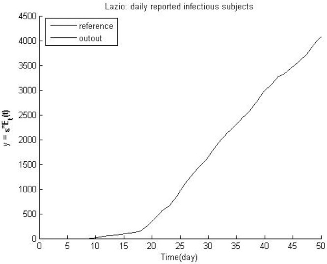
Fig. 3 shows the input data that is collected from daily reports in Hubei (China) and Lazio (Italy). It is validated for 25 days (Dec 29, 2019 to Jan 23, 2020) in Hubei and 50 days in Lazio (Feb 24, 2020 to Apr 14, 2020) of the outbreak [17].

Fig. 3.

Validated data of China and Lazio outbreak.

Fig. 4 presents the open loop responses of the open loop system such as the states of the system, the tracking properties of the system and the phase-plane of the system. Apparently, the system is unstable because the epidemic is out of control and the virus is speared through people in nonlinear way.

Fig. 4.

Open loop system responses in Hubei and Lazio.

3.2. Closed loop system of Hubei (China) reports

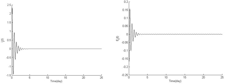
In this subsection, the results of the controlled COVID-19 system are presented which based on the daily reports of the government in Hubei (China). Fig. 5 shows the stabilization properties of the system states ($I_t(t)$, $E_t(t)$) with initial condition ($I_t\left(0\right)=0.25$ and $E_t\left(0\right)=0.75$).

Fig. 5.

Stabilization properties of the system states ($I_t(t)$, $E_t(t)$).

Fig. 6 presents the system state trajectories after applying the controller (Eq. (30)). However, the shadow parts caused by the $sign(\bullet )$ term of the controller.

Fig. 6.

the system state trajectories ($I_t(t)$, $E_t(t)$).

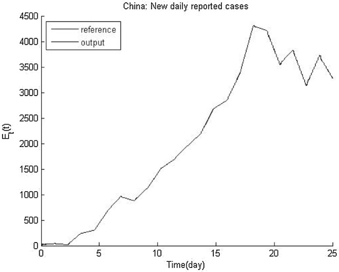
Fig. 7 illustrates the exact tracking property trajectory of the COVID-19 controlled system. Fig. 8 explains the phase-plane of the system which is started and ended at zero point; it indicates that the zero point is stable equilibrium point of the system.

Fig. 7.

Tracking properties of the system.

Fig. 8.

Phase-plane of the COVID-19 system.

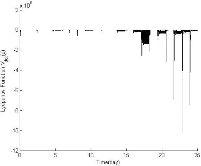
Fig. 9 shows the control action ($\beta (u\left(t\right))$) that is started at high point because of the high number of the infected cases at the beginning of the COVID-19 outbreak. Fig. 10 proves that the proposed controller (Eq. (30)) successfully stabilized the COVID-19 system.

Fig. 9.

Control action $\beta (u\left(t\right))$ of the system.

Fig. 10.

Time-derivative of the LQF.

3.3. Closed loop system of Lazio (Italy) reports

In this subsection, the results of the controlled COVID-19 system are presented that based on the daily reports of the government in Lazio (Italy). Fig. 11 represents the stabilized system states ($I_t(t)$, $E_t(t)$) with initial condition ($I_t\left(0\right)=0.25$ and $E_t\left(0\right)=0.75$. It is shown that the potential effect of the proposed controller (Eq. (30)) in stabilizing the system effectively.

Fig. 11.

Stabilization properties of the system states ($I_t(t)$, $E_t(t)$).

Fig. 12 presents the trajectories of the system states after applying the proposed controller (Eq. (30)).

Fig. 12.

the system state trajectories ($I_t(t)$, $E_t(t)$).

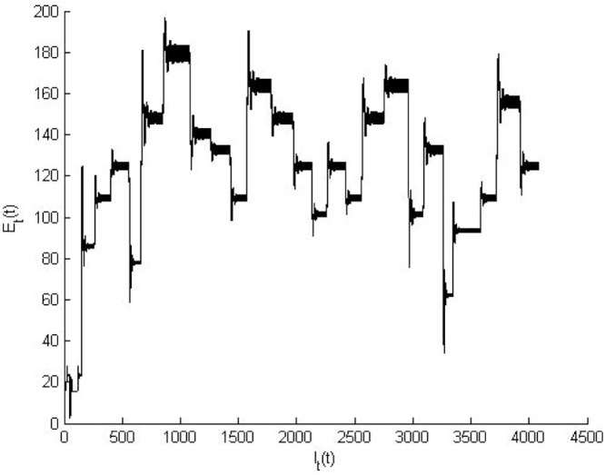
Fig. 13 illustrates the tracking property trajectory of the COVID-19 system after applying the proposed controller. Fig. 14 explains the phase-plane of the COVID-19 system which proves that the zero point is stable equilibrium point of the system. Furthermore, the shadow parts caused by the $sign(\bullet )$ term of the controller.

Fig. 13.

Tracking properties of the system.

Fig. 14.

Phase-plane of the system.

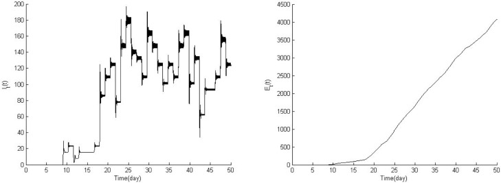
Fig. 15 shows the control action ($\beta (u\left(t\right))$) that is jumped at high point at the day 10 because of the infected cases started to increase in this day in Lazio outbreak. Fig. 16 shows and proves that the proposed controller (Eq. (30)) successfully stabilized the COVID-19 system.

Fig. 15.

Control action $\beta (u\left(t\right))$ of the system.

Fig. 16.

Time-derivative of the LQF.

Fig. 17 shows the error convergence of the cost function after applying the Most Valuable Player Algorithm (MVPA) in order to optimize the parameters of the proposed controller (Eq. (30)).

Fig. 17.

Convergence properties of the MVPA.

It is shown that 3 iterations are enough to achieve the convergence property to minimize the cost function. It is worth to mention that an iteration is corresponding to the day unit of the COVID-19 epidemic.

4. Discussion

The previous results have shown that this strategy (mathematical-engineering strategy) can work in parallel with other existing strategies (suppression and mitigation) to control and reduce the separation of the COVID-19 epidemic. However, this strategy may not be effective as the vaccine of the COVID-19 is not been invented yet. In addition, these results are valid for a certain period of time for both cities (Hubei and Lazio) which can be applied for any other place in any time if the required data is available. In addition, the results proved the effectiveness of the proposed control algorithm from control theory prospective which is interpreted by the performance improvements, stability achievement, the optimality of the parameters and the robustness of the controlled COVID-19 system. Eventually, this strategy (robust control algorithm) can be used to control and reduce the separation of any other epidemic outbreak in the future if the required data and model of this epidemic is available.

5. Conclusions

In this work, a novel robust control algorithm has been proposed in order to involve the control theory concepts to present a solution to the COVID-19 epidemic alongside with suppression and mitigation strategies. In addition, the COVIS-19 nonlinear system has been compensated using the proposed control algorithm. Then, the Variable Transformation Technique (VTT) has been successively applied to simplify the COVID-19 nonlinear system to fit the analysis procedure. After that, the optimal parameters of the proposed control algorithm have been obtained using the Most Valuable Player Algorithm (MVPA). Finally, the simulation results have explained the ability of the proposed control algorithm in compensating the COVID-19 system based on the daily reports in both Hubei (China) and Lazio (Italy).

Author statement

Musadaq A. Hadi: substantial contribution to conception and design; substantial contribution to acquisition of data; substantial contribution to analysis and interpretation of data; drafting the article; critically revising the article for important intellectual content; final approval of the version to be published.

Hazem I. Ali: critically revising the article for important intellectual content; final approval of the version to be published.

References

- 1.WHO . 2020. Coronavirus Disease (COVID-2019) Situation Reports.https://www.who.int/emergencies/diseases/novel-coronavirus-2019/situation-reports [Accessed 19 June 2020] [Google Scholar]
- 2.Lu R., Zhao X., Li J., Niu P., Yang B., Wu H. Genomic characterisation and epidemiology of 2019 novel coronavirus: implications for virus origins and receptor binding. Lancet. 2020;395:565–574. doi: 10.1016/S0140-6736(20)30251-8. [DOI] [PMC free article] [PubMed] [Google Scholar]
- 3.Cai Q., Yang M., Liu D., Chen J., Shu D., Xia J., Liao X., Gu Y., Cai Q., Yang Y., Shen C. Experimental treatment with Favipiravir for COVID-19: an open-label control study. Eng. J. 2020 doi: 10.1016/j.eng.2020.03.007. [DOI] [PMC free article] [PubMed] [Google Scholar]
- 4.Riou J., Althaus C. Pattern of early human-to-human transmission of Wuhan 2019 novel coronavirus (2019-nCoV), December 2019 to January 2020. Eurosurveillance. 2020;25 doi: 10.2807/1560-7917.ES.2020.25.4.2000058. [DOI] [PMC free article] [PubMed] [Google Scholar]
- 5.Liu Y., Gayle A., Wilder-Smith A., Rocklöv J. The reproductive number of COVID-19 is higher compared to SARS coronavirus. J. Travel Med. 2020;27 doi: 10.1093/jtm/taaa021. [DOI] [PMC free article] [PubMed] [Google Scholar]
- 6.Yu P., Zhu J., Zhang Z., Han Y. A familial cluster of infection associated with the 2019 novel coronavirus indicating possible person-to-person transmission during the incubation period. J. Infect. Dis. 2020;(221):1757–1761. doi: 10.1093/infdis/jiaa077. [DOI] [PMC free article] [PubMed] [Google Scholar]
- 7.KRR G., Casella F. 2020. Non-Pharmaceutical Interventions (NPIs) to Reduce COVID-19 Mortality. SSRN E. J. [DOI] [PMC free article] [PubMed] [Google Scholar]
- 8.Hunter D. Covid-19 and the stiff upper lip — the pandemic response in the United Kingdom. N. Engl. J. Med. 2020;382:e31. doi: 10.1056/NEJMp2005755. [DOI] [PubMed] [Google Scholar]
- 9.James A., Hendy S., Plank M., Steyn N. 2020. Suppression and Mitigation Strategies for Control of COVID-19 in New Zealand. [DOI] [Google Scholar]
- 10.Rocklov J. 2020. COVID-19 Health Care Demand and Mortality in Sweden in Response to Non-Pharmaceutical (NPIs) Mitigation and Suppression Scenarios. [DOI] [PMC free article] [PubMed] [Google Scholar]
- 11.Rad H., Badi A. 2020. A Study on Control of Novel Corona-Virus (2019-nCoV) Disease Process by Using PID Controller. [DOI] [Google Scholar]
- 12.Hethcote H. The mathematics of infectious diseases. Siam Rev. 2000;42:599–653. [Google Scholar]
- 13.Xu C., Lei H., Li J., Ye J., Zhang D. Adaptive neural control for nonaffine pure-feedback system based on extreme learning machine. Math Probl. Eng. 2019:1–13. doi: 10.1155/2019/5613212. [DOI] [Google Scholar]
- 14.Ali H., Hadi M. Optimal nonlinear controller design for different classes of nonlinear systems using black hole optimization method. Arab. J. Sci. Eng. 2020;45:7033–7053. doi: 10.1007/s13369-020-04650-z. [DOI] [Google Scholar]
- 15.Rahimian M., Tavazoei M. Improving integral square error performance with implementable fractional-order PI controllers. Optim. Contr. Appl. Met. 2013;35:303–323. doi: 10.1002/oca.2069. [DOI] [Google Scholar]
- 16.Bouchekara H. Most Valuable Player Algorithm: a novel optimization algorithm inspired from sport. Oper. Res. 2017;20:139–195. doi: 10.1007/s12351-017-0320-y. [DOI] [Google Scholar]
- 17.Casella F. 2020. Can the COVID-19 Epidemic Be Controlled on the Basis of Daily Test Reports?https://arxiv.org/pdf/2003.06967v3.pdf [Accessed 5 July 2020] [Google Scholar]