Figure 2, Improvements in deconvolution and registration accelerate the processing of multiview light-sheet datasets.

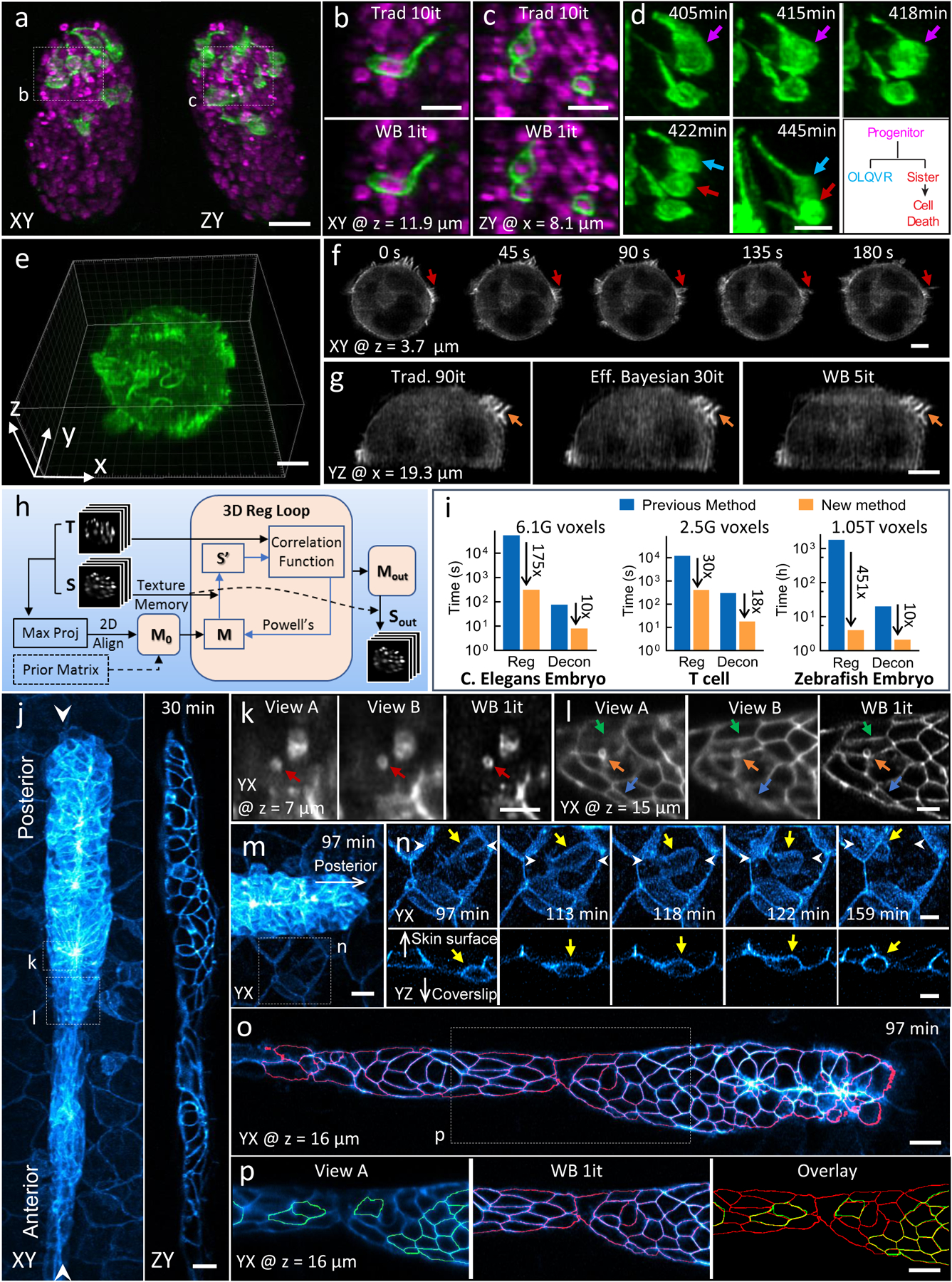
a) Lateral (left) and axial (right) maximum intensity projections demonstrate isotropic reconstructions of C. elegans embryos expressing neuronal (green, GFP-membrane marker) and pan-nuclear (magenta, mCherry-histone) markers. Images were captured with diSPIM, and deconvolution was performed using the Wiener-Butterworth (WB) filter. See also Supplementary Video 4. b, c) Higher magnification single slices from dotted rectangular regions in a), emphasizing similarity between reconstructions obtained with traditional Richardson-Lucy deconvolution (‘trad’) and WB deconvolution. Iterations (it) for each method are displayed. d) Higher magnification maximum intensity projection view of neuronal dynamics, indicating neurite extension and terminal cell division for progenitor (purple arrow), OLQVR (blue arrow) and apoptotic sister cell (red arrow). See also lower right schematic and Supplementary Video 5. e) WB reconstruction of Jurkat T cell expressing EGFP-actin, raw data captured in a quadruple-view light-sheet microscope. f) Selected slices 3.7 μm from the coverslip surface. Indicated time points display fine actin dynamics at the cell periphery. See also Supplementary Video 6. g) Axial slice through sample, indicating close similarity between traditional, efficient Bayesian, and WB deconvolution with iteration number as indicated. h) Schematic of GPU-based 3D registration used for multiview fusion. Example inputs are two 3D images, referred as the source (S, image to be registered) and target image (T, fixed image). Maximum intensity projections of the input 3D images are used for preliminary alignment and to generate an initial transformation matrix (M₀). Alternatively, a transformation matrix from a prior time point is used as M₀. A 3D registration loop iteratively performs affine transfomations on S (which is kept in GPU texture memory for fast interpolation), using Powell’s method for updating the transformation matrix by minimizing the correlation ratio between the transformed source (S’) and T. i) Bar graphs showing time required to process the datasets (file I/O not included) in this figure (left, middle and right columns corresponding to datasets in a, e and j, respectively, with voxel count as indicated) conventionally and via our new methods. The conventional registration method was performed using an existing MIPAV plugin (see Methods) using CPUs while the new registration method was performed using GPUs. Both deconvolution methods were performed with GPUs. Note log scale on ordinate, and that the listed times apply for the entire time series in each case (the total time for the conventional registration method on the zebrafish dataset was extrapolated from the time required to register 10 time points). j) Representative lateral (left, maximum intensity projection) and axial (right, single plane corresponding to white arrowheads in left panel) images showing 32-hour zebrafish embryo expressing Lyn-eGFP under the control of the ClaudinB promoter, marking cell boundaries within and outside the lateral line primordium. Images were captured with diSPIM, Wiener-Butterworth reconstructions are shown. Images are selected from the volume 30 minutes into the acquisition, see also Supplementary Video 7. k, l) Higher magnification views of dotted rectangles in j), emphasizing improvement in resolving vesicles (red, orange arrows) and cell boundaries (green, blue arrows) with WB deconvolution compared to raw data. Note that k, l are rotated 90 degrees relative to j. m) Higher magnification view of leading edge of lateral line, 97 minute into the acquisition. n) Higher magnification view of dotted rectangular region in m), emphasizing immune cell (yellow arrow) migration between surrounding skin cells. White arrowheads are provided to give context and the white arrows point towards skin surface and coverslip. Top row: maximum intensity projection of lateral view, bottom row: single plane, axial view. See also Supplementary Video 8. o) Lateral slice through primordium, with automatically segmented cell boundaries marked in red. See also Supplementary Video 9. p) Higher magnification view of dotted rectangle in o), showing differential segmentation with raw single-view data (green, left) vs. deconvolved data (red, middle). Overlay at right shows common segmentations (yellow) vs. segmentations found only in the deconvolved data (red). Note that ‘z’ coordinate in j-p is defined normal to the coverslip surface. Scale bars: 10 μm in a), m), o) and p); 5 μm in all other panels. Experiments were repeated on similar datasets at least 3 times for a)-d), 2 times for e)-g) and j)-p), with similar results obtained each time; representative data from a single experiment are shown.