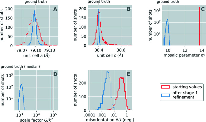
Figure 3.

Stage 1 refinement results for 2023 exposures. During stage 1 refinement images are refined separately, resulting in a unique scale factor G_s, mosaic domain parameter m_s, unit cell matrix B _s and rotation matrix U _s for each crystal. Starting values are shown in red, and optimized values after stage 1 refinement are shown in blue. (a) and (b) Unit cell edges a and c. Initial values come from the DIALS indexing program (Winter et al., 2018 ▸). Despite all crystals having the same unit cell (a = 79.1, c = 38.4 Å), the indexing results returned a distribution of cells. The unit cell a-edge refined to a median value of 79.097 Å, which is 0.003 Å different from the ground truth value. By modeling each shot with its known photon energy spectra, we indeed recovered a value of 79.100 Å for the median a-edge; however, the added accuracy was not worth the computational cost of simulating each energy in the spectrum separately. This is why we elected to use the reduced equation (16) to model the Bragg scattering. (c) Dimensionless mosaic parameters m_s. The initial value of 13.7 resulted from analyzing the mosaic domain size distribution deduced by DIALS during indexing. The median value of m after the stage 1 refinement (9.92) differs from the ground truth by 0.08. We hypothesize that this is because the synthetic data included a mosaic texture distribution that increased the size of the Bragg spots in reciprocal space. Smaller values of m correspond to larger Bragg spots, hence the model is likely trying to compensate for the absence of any mosaic texture in equation (16). (d) Dimensionless scale factors G_s. To compare with the ground truth, all scale factors G_s were divided by a factor k ² where k = 3.68 is the scale factor which minimizes R _GT shown in equation (28). Initially we let all G_s be 10⁶, which when divided by k ² gives a value of 7.4 × 10⁴ as indicated by the red bar. (e) Misorientation of each crystal from its ground truth. During actual XFEL data collection one can never know this quantity, but synthetic data provides a unique opportunity to use this quantity as a proxy for model accuracy. We approach the optimal model when all . Note, the vertical axes in (c) and (d) and the horizontal axes in (d) and (e) are on logarithmic scales.