Does the “Reticular Lamina Nonlinearity” Contribute to the Basal DPOAE Source?

Abstract

The spatial extent of the cochlear region that actually contributes to the DPOAE signal measured in the ear canal may be evaluated experimentally using interference tones or computed numerically using nonlinear cochlear models. A nonlinear transmission-line cochlear model is used in this study to evaluate whether the recently reported nonlinear behavior of the reticular lamina (RL) over a wide basal region may be associated with generation of a significant distortion product otoacoustic emission (DPOAE) component. A two-degrees-of-freedom 1-D nonlinear model was used as discussed by Sisto et al. (2019), in which each local element consists of two coupled oscillators, roughly representing the basilar membrane (BM) and the RL. In this model, the RL shows a strongly nonlinear response over a wide region basal to the characteristic place, whereas the BM response is linear outside the narrow peak region. Such a model may be considered as that using the minimal number of degrees of freedom necessary to separately predict the motion of the BM and RL, while preserving important cochlear symmetries, such as the zero-crossing invariance of the impulse response. In the numerical simulations, the RL nonlinearity generates indeed a large intracochlear distortion product source, extended down to very basal cochlear regions. Nevertheless, due to the weak and indirect coupling between the RL motion and the differential fluid pressure in the basal part of the traveling wave path, no significant contribution from this mechanism is predicted by the model to the generation of the DPOAE signal that is eventually measured in the ear canal.

Introduction

Recent experiments on small mammals (e.g., Lee et al. 2015; Dewey et al. 2019; Ren and He 2020) have shown nonlinear response of the RL over a large cochlear longitudinal region, basal to the resonant place. This well-established observation might suggest that the RL nonlinear response could be responsible for the generation of a corresponding basal DPOAE component. The generation of distortion products on the RL in the basal region of the cochlea is also related to SFOAE suppression and the consequent generation of residuals by high-frequency tones (Siegel 2018). On the other hand, the localization of the DPOAE sources within a frequency-specific region, e.g., for the 2f₁-f₂ distortion product (DP), around the characteristic resonant place (CP) of frequency f₂, is supported by the sharpness of the DPOAE suppression tuning curves (STCs, see, e.g., Abdala et al. 1996) and by the high diagnostic power and frequency specificity of DPOAE-based hearing diagnostic techniques.

DPOAE response is assumed to be generated by two mechanisms (e.g., Shera and Guinan 1999). Focusing on the DP at frequency f_DP = 2f₁-f₂, any odd-order nonlinear distortion generates backward and forward traveling waves (TWs) at frequency 2f₁-f₂, called intracochlear distortion product (IDP) waves, with a local source strength proportional to a cubic function of the local transverse displacement/velocity at the stimulus frequencies f₁ and f₂. This strength is generally assumed to be significantly large only within the so-called overlap region, where response is sufficiently strong at both primary frequencies. It is roughly localized near the CP of frequency f₂, and its spatial extension towards the base depends on the stimulus level and on the stimulus frequency ratio r = f₂/f₁ (e.g., Sisto et al. 2018). The overlap region may be quantitatively defined as that where the DP local source strength differs from its maximum value by less than, e.g., 10 dB. At high stimulus levels and/or small ratios, the large spatial extension of this region implies a large phase dispersion among the backward DP wavelets generated at different places, resulting in decreased DPOAE response due to destructive interference.

The IDP forward wave eventually reaches its resonant region, where it is amplified and partially reflected by cochlear roughness. This linear coherent reflection mechanism generates a second backward TW at the f_DP frequency, which adds vectorially to the distortion component, to generate the DPOAE measured in the ear canal. Due to the wave- and place-fixed nature of, respectively, the distortion and reflection mechanisms (Shera and Guinan 1999), the phase difference between the two components is a monotonic function of frequency, so interference between them yields the so-called DPOAE spectral fine structure.

Several studies (e.g., Martin et al. 2010, 2016) have investigated the spatial distribution of IDP sources and its relation with the DPOAE measured in the ear canal. This relation is not straightforward, because one must consider interference among backward DP wavelets of different phase, coming from wide cochlear regions. Indeed, Martin et al. (2010) showed that in rabbits, high-frequency interference tones (IT) may either suppress or enhance the DPOAE, as expected if interference effects have a dominant role. The spatial extent of the basal generation region may affect the diagnostic potential of DPOAEs because in hearing-impaired subjects, a localized cochlear damage could, similarly to an IT, either enhance or suppress the total DPOAE level, depending on the width of the damaged region and on the phase of the local DP generators. Martin et al. suggested that measuring DPOAEs with and without ITs could improve the power of DPOAE-based hearing diagnostic techniques by reducing the uncertainty associated with these interference phenomena. On the other hand, Withnell and Lodde (2006) had found no evidence for DPOAE basal sources in guinea pigs, by causing frequency-specific damage in the basal part of the cochlea.

In this framework, the hypothesis of a significant DPOAE generation at very basal places (one octave or more above f₂) associated with the RL nonlinearity would significantly change the above-described picture, and it would be rather inconsistent with the sharpness of the DPOAE STCs and with the high-frequency specificity and diagnostic power of DPOAE-based hearing diagnostic techniques.

Nonlinear cochlear models solved in time domain allow one to monitor the generation of an intracochlear TW at the distortion product frequency, and its propagation in the differential fluid pressure, automatically including all generation, propagation, suppression, and interference phenomena that contribute to yielding the stationary DP response over the whole cochlea. We recall here that the DP differential pressure at the cochlear base is the physical quantity that actually drives the stapes backwardly, being therefore directly related to the DPOAE response measured in the ear canal (see, e.g., Talmadge et al. 1998).

A nonlinear cochlear model may evaluate the distributed generation of the IDP, its backward propagation to the base, the transmission through the middle ear of the DP, and the generation of the DPOAE in the ear canal. Finite element models (e.g., Sasmal and Grosh 2019) may be effectively used for this purpose, being able to describe the local motion of all the cochlear structures, but they may be computationally expensive and are characterized by a large number of free parameters, whose tuning limits their predictive power.

The 1-D transmission-line cochlear models are rough schematizations of the anatomy of the OC, using a lumped parameter representation involving point-like masses interacting between them and with the differential fluid pressure. The advantage of such a simplified formulation, a part of the short computing time, is twofold: analytical solutions in the low stimulus level limit easily provide physical insight, allowing one to understand the meaning and the consequences of each parameter choice, and the number of the model free parameters is small.

The minimal degree of complexity necessary for a transmission-line model to highlight the different roles of the BM and of the RL is provided by two-degrees-of-freedom (2DOF) models. An obvious limitation of this approach is due to schematizing a complex structure as the OC, in which inertia, elasticity, damping, and nonlinear forces are distributed as continuous variables in each infinitesimal volume element, with two point-like masses in which all inertia is concentrated, interacting between them and with the differential fluid pressure.

We used a new 2DOF nonlinear 1-D transmission line cochlear model (Sisto et al. 2019), in which two oscillators, which can be roughly identified with the BM and the RL, are coupled by an internal nonlinear force representing the action of the outer hair cells (OHC) amplification system. The BM is also directly coupled to differential pressure through fluid incompressibility.

A real-zero version of the model was used, in which the normal modes of the system consist of a single oscillatory mode and a pure damping mode. In the low stimulus level linear limit, the transfer function at each cochlear place has just one complex pole, whose imaginary part represents the local resonant frequency, while the other pole (as well as the zero) is real; i.e., it has only a damping effect (see Fig. 8 in Sisto et al. 2019). This model has other interesting physical properties, such as approximately respecting the zero-crossing invariance of the BM impulse response, and, particularly relevant for the issue discussed in this study, the fact that the RL shows nonlinear behavior over a spatial (or, equivalently, frequency) range much wider than the spatial extent (bandwidth) of the activity peak of the BM. The model was used to compute the response at the DP frequency in terms of BM and RL velocity and of differential fluid pressure, as a function of the longitudinal cochlear coordinate x.

As mentioned before, 2DOF lumped parameter models cannot predict where the wideband nonlinear behavior is localized within the structures actually existing between the BM and the RL. Nevertheless, the real-zero 2DOF model (Sisto et al. 2019) predicts that the nonlinear response over an extended basal region is a property of the second mass only. Whatever this “effective” second mass actually represents (a suitable spatial average of the inertia of the structures above the BM, effectively localized somewhere within them), its relevant physical properties are as follows: (1) being the inertial element that is not directly coupled to the differential pressure, but only to the first mass (the BM), and (2) being weakly (or not at all) tonotopically tuned.

The potential dynamical role of the tectorial membrane (TM, considered here a rigid wall) in the propagation of DP waves is also neglected in the model, as well as the possible weak coupling of the RL motion to the differential pressure. We remark that other 2DOF transmission-line models (e.g., de Boer 1990) allow interaction between the pressure in the scalae and the BM, RL, and TM motion, yielding multiple, mutually interacting TWs.

The presence of a second mechanism of generation by coherent reflection in the resonant region of the DP, which further complicates the DPOAE phenomenology, was also neglected in this study. The reflection component is generally smaller than the distortion component, except at very small stimulus levels and/or small ratios f₂/f₁ (see, e.g., Martin et al. 2010, 2016; Botti et al. 2016), so it seems reasonable, for clarity, to focus on the so-called nonlinear distortion component of the DPOAE, using a cochlear model without roughness. Including roughness in the model would have yielded the characteristic fine structure of DPOAE spectra, and a meaningful analysis would have required performing a large number of simulations varying the stimulus frequencies with high-frequency resolution in order to unmix the DPOAE components.

Model

A comprehensive description of the real-zero model, and of its formulation using state space variables (Elliott et al. 2007), is given elsewhere (Sisto et al. 2019). In this 1-D transmission-line box model, each cochlear element is schematized as a system of two oscillators, 1 and 2 (identifiable, respectively, with the BM and the RL). Each oscillator is characterized by its lumped parameters M_i, C_i, and K_i, with i = 1,2, representing mass, damping, and stiffness per unit surface, while the transverse displacement of the two masses is described by the kinematic variables ξ_i. The two oscillators are coupled by passive elastic and damping internal forces (parameterized by the coefficients K₃ and C₃). The BM is sharply tuned and directly coupled to the differential pressure p of the perilymph, while the other oscillator can be roughly tuned (or not tuned at all) and directly coupled to the BM only. In the nonlinear model, when a displacement component at the DP frequency is nonlinearly generated on the BM, it is locally fed to the differential pressure through fluid incompressibility, which is an implicit ingredient of the pressure propagation equation (the first of Eq. 1).

The OHC mechanism is represented by an additional internal nonlinear coupling force between the BM and the RL, including terms proportional to both relative displacement and relative velocity of the two masses.

The model equations can be written as

$$\{\begin{array}{c}\frac{{\partial }^{2}p}{\partial x^2}=-\frac{2\rho }{H}{\ddot{\xi }}_1\\ M_1{\ddot{\xi }}_1+C_1{\dot{\xi }}_1+K_1{\xi }_1=-p-C_3\left({\dot{\xi }}_1-{\dot{\xi }}_2\right)-K_3\left({\xi }_1-{\xi }_2\right)+K_{\mathit{nl}}\left({\xi }_1-{\xi }_2\right)+C_{\mathit{nl}}\left({\dot{\xi }}_1-{\dot{\xi }}_2\right)\\ M_2{\ddot{\xi }}_2+C_2{\dot{\xi }}_2+K_2{\xi }_2=C_3\left({\dot{\xi }}_1-{\dot{\xi }}_2\right)+K_3\left({\xi }_1-{\xi }_2\right)-K_{\mathit{nl}}\left({\xi }_1-{\xi }_2\right)-C_{\mathit{nl}}\left({\dot{\xi }}_1-{\dot{\xi }}_2\right)\end{array}.$$ 1

where ρ is the density of the perilymph, H and L are, respectively, the height and length of the cochlear cavity, and K_nl and C_nl are nonlinear functions of the relative displacement and velocity describing the OHC mechanism:

$$\{\begin{array}{c}{K}_{\mathsf{nl}}=K_4\left(\mathsf{1}-\mathsf{tanh}{\left(\frac{{\left({\xi }_1-{\xi }_2\right)}^2}{{\xi }_{\mathit{sat}}^2}+\frac{{\left({\dot{\xi }}_1-{\dot{\xi }}_2\right)}^2}{v_{\mathit{sat}}^2}\right)}^{\alpha }\right)\\ C_{\mathsf{nl}}=C_4\left(\mathsf{1}-\mathsf{tanh}{\left(\frac{{\left({\xi }_1-{\xi }_2\right)}^2}{{\xi }_{\mathit{sat}}^2}+\frac{{\left({\dot{\xi }}_1-{\dot{\xi }}_2\right)}^2}{v_{\mathit{sat}}^2}\right)}^{\alpha }\right)\end{array}$$ 2

where ξ_sat and v_sat are the nonlinear saturation displacement and velocity scales, respectively. For a full list of parameter values, see Table 1. In the small-displacement linear limit, K_nl = K₄ and C_nl = C₄, while on the opposite limit, i.e., the saturation one, K_nl = 0 and C_nl = 0. These internal force terms are nonlinearly dependent on the local instantaneous relative displacement and velocity between BM and RL. In the small-displacement linear limit, one can define the local characteristic resonant frequency of the BM as

$$\mathit{CF}\left(x\right)=\frac{1}{2\pi }\sqrt{\frac{K_1\left(x\right)+K_3\left(x\right)-K_4\left(x\right)}{M_1\left(x\right)}}$$ 3

Table 1.

Parameters of the nonlinear model used in the simulations

M1(x)	0.03 kg/m2
M2(x)	0.3M1
K1(x)	1.1·1010exp(−400x)
K2(x)	0.055(M2/M1)K1
K3(x)	0.045(M2/M1)K1
K4(x)	0.02(M2/M1)K1
C1(x)	6500exp(−200x)
C2(x)	2(M2(K2 + K3−K4))0.5−(C3−C4)
C3(x)	0.3C1
C4(x)	0.93C1
ξsat	1.4·10−8 m
vsat	1.8·10−4 m/s
L	0.025 m
H	0.007 m
ρ	1000 kg/m3

The parameter α was tuned to 1/3, in order to get a realistic slope of the DPOAE I/O functions (about 1 dB/dB) in the low stimulus level limit. In the model, the differential pressure p acts only on the mass M₁ (the BM), because only the BM is in direct contact with the perilymph. For the same reason, the counter-reaction on the fluid pressure longitudinal gradient due to fluid incompressibility is associated with the BM motion only. Any indirect effect of p on M₂ (the RL) through the Reissner’s membrane and the endolymph is assumed here to be negligibly small, compared with that of the internal forces (active and passive) between BM and RL. The same assumption is made in several other 2DOF models (Lu et al. 2006; Liu and Neely 2009; Elliott et al. 2017). The feedback forces are treated as internal forces between the two masses, respecting therefore the action-reaction principle. Newton’s third law (the action/reaction principle) ensures that the internal (both OHC and passive) forces on the BM and RL are equal and opposite to each other, but this fact does not imply that the nonlinear behavior must be similar for them. Indeed, the two oscillators have different impedances, as we will show in some detail. In the Laplace linear formalism, each time derivative yields a simple multiplication by the complex Laplace variable s. The differential Eq. (1) becomes an algebraic equation for the Laplace-transformed variables, pressure, and displacements. The two oscillators’ impedances are written as

$$Z_i=s{M}_i+C_i+\frac{K_i}{s}.$$ 4

As regards the internal force terms, in a linear version of the model, they may be represented by the internal impedance:

$$Z_{\mathit{int}}=C_3-\beta C_4+\frac{\left(K_3-\beta K_4\right)}{s}$$ 5

where β, homogenously variable (independent of x) between 0 and 1, parameterizes a family of linear models with different degrees of the OHC local force strength (see Fig.1). In the nonlinear model, this strength is not constant along x, because it depends on the local BM and RL relative displacement/velocity.

Fig. 1.

BM (blue line), RL (red), and internal (black) impedance magnitudes for f₂ = 1 kHz, for β variable in the range (0:1) with 0.2 steps, as a function of the longitudinal coordinate x, expressed in dimensionless units as the ratio between f₂ and the local characteristic resonance frequency CF(x). This ratio is equal to unity at the characteristic place of f₂, CP(f₂). Line thickness increases with increasing β

The three impedances are connected to the differential pressure as in the equivalent circuit of Fig. 2. This circuit representation yields, in the linear limit, a simple expression for the BM and RL admittances, defined as the ratios of the Laplace-transformed velocity to the Laplace-transformed pressure, which may help understanding what happens as the OHC impedance terms K_nl and C_nl vary in the nonlinear regime:

$$\{\begin{array}{c}{Y}_{\mathit{BM}}=\frac{\left(Z_{\mathit{int}}+Z_2\right)}{Z_1{Z}_2+Z_1{Z}_{\mathit{int}}+Z_2{Z}_{\mathit{int}}}={\left(Z_1+\frac{Z_2{Z}_{\mathit{int}}}{Z_{\mathit{int}}+Z_2}\right)}^{-1}\\ Y_{\mathit{RL}}=\frac{Z_{\mathit{int}}}{Z_1{Z}_2+Z_1{Z}_{\mathit{int}}+Z_2{Z}_{\mathit{int}}}=Y_{\mathit{BM}}\frac{Z_{\mathit{int}}}{Z_{\mathit{int}}+Z_2}=Y_{\mathit{BM}}{\left(1+\frac{Z_2}{Z_{\mathit{int}}}\right)}^{-1}\end{array}$$ 6

Fig. 2.

Lumped elements circuit representation of the local coupling among differential pressure, BM and RL (whose impedance elements are labeled as 1 and 2, respectively), including internal linear and nonlinear coupling (elements labeled as 3 and nl, respectively) between BM and RL

The two admittances are shown in Fig. 3, as a function of the longitudinal coordinate x, for β variable in the [0:1] interval with 0.2 steps. One may easily note that the nonlinear behavior of the RL admittance extends to very basal regions and that the dependence on β is non-monotonic.

Fig. 3.

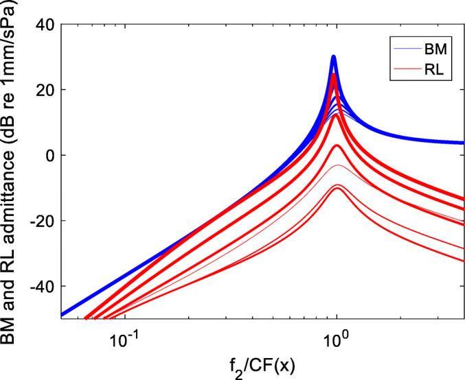
BM (solid lines) and RL (dashed) admittance magnitudes as functions of the longitudinal coordinate x, expressed in dimensionless units, in the linear approximation, for β variable in the range [0:1] with 0.2 steps. Line thickness increases proportional to β. Note that the admittances are non-monotonic functions of β, due to the competition between internal force terms of opposite sign. Note also that in the basal region, the BM admittance scales as the inverse square of the local CF (its slope is approximately 40 dB/decade)

Requesting that the zeros of the 2DOF BM admittance be real enforces the zero-crossing symmetry (Sisto et al. 2019). Another consequence of imposing the real-zero condition is getting a particular pair of normal modes: a single high-Q oscillatory mode and a pure damping mode (of critical or supercritical damping). Indeed, one of the poles of the underlying linear system is also real, so it does not yield a second resonant frequency (which would have been associated with its imaginary part).

The model was solved in time domain using the state space formalism (Elliott et al. 2017), yielding a state vector consisting of velocity and displacement of BM and RL at each cochlear place as a function of time. Differential pressure is also computed from the model equations. Fourier transforms of the time domain solution at any cochlear place yield the response of the system as a function of two variables, frequency and place. In these simulations, N = 500 elements along the longitudinal direction were used. Such a small number of cochlear elements are sufficient to get accurate simulations of the DP generation and transmission, whereas it would have been insufficient to correctly evaluate the effect of roughness, which is not included in the model.

Results

For cochlear DP generation simulations, two sinusoidal stimuli were used at fixed frequencies f₁ and f₂, with f₂ = 2 kHz and r = 1.3, with the level L₁ of the lower-frequency stimulus set to 10 dB above L₂, which was varied over a 60 dB range with 10 dB steps, between 25 and 85 dB SPL. The time domain solution was Fourier transformed, yielding, for each frequency, the amplitude and phase of the response as a function of the longitudinal coordinate x. In a DPOAE generation simulation, one is interested in the response at the frequencies f₁, f₂, and f_DP = 2f₁-f₂.

In Fig. 4 (left), the pure tone response gain, defined as the ratio of the local response at frequency f₂ to that at the cochlear base, is shown, for the BM velocity (blue) and the RL velocity (red), for seven stimulus levels varying in the 25–85 dB range, as functions of the longitudinal coordinate x, expressed in dimensionless units as the ratio between f₂ and the local characteristic resonance frequency CF(x). This dimensionless unit is easily visually interpreted in terms of logarithmic intervals along the BM, as, e.g., a local ratio of 0.5 means that the local resonant CF is 2f₂. The RL nonlinear behavior extends significantly towards the base, over a wide stimulus level range, whereas the BM response is linear away from the peak region, which may be quantitatively defined as that where the response level differs from the peak level by less than, e.g., 10 dB.

Fig. 4.

(Left) BM (blue) and RL (red) pure tone response gain at frequency f₂ = 2 kHz, as functions of the longitudinal coordinate x, for stimulus levels varying in the range of 25–85 dB SPL with 10 dB steps. The RL response grows nonlinearly over a wide region basal to the characteristic place of f₂. The pressure gain (green) is also shown. (Right) Local magnitude of the BM (blue) and RL (red) velocity and differential pressure (green), at the frequency f_DP = 2f₁-f₂, as functions of the longitudinal coordinate x, generated by two tones f₁ and f₂, with L₁ = L₂ + 10 dB and L₂ varied between 25 and 85 dB SPL with 20 dB steps. Here, the local velocity is shown in dB relative to 1 nm/s, while pressure is in dB is 200 pPa, i.e., dB SPL + 40 dB. Line thickness increases with increasing stimulus level. The RL response at f_DP is larger than that of the BM over a region basal to CP(f₂), whose spatial extent increases with increases stimulus level. All simulations are performed with constant f₂ = 2 kHz and constant r = 1.3. A dimensionless spatial coordinate is used as abscissa, as in Sisto et al. (2019), which equals unity at the characteristic place of the stimulus frequency f₂ = 2 kHz, corresponding to the apical edge of the overlap region where nonlinear distortion generation takes place

In the right panel of Fig. 4, the response at f_DP is shown as a function of x for the BM velocity (blue), the RL velocity (red), and the differential pressure (green). On the RL, a strong nonlinear response at frequency f_DP is predicted at high stimulus levels over a wide basal region encompassing up to three octaves (at the highest stimulus level) in terms of local CF. On the other hand, the effect of this basal DP generation on the DPOAE response is expected to be negligible. To understand that, one should consider that the physical entity mechanically coupled to the stapes is the fluid pressure, which, in the model, is not directly coupled to the RL motion but only to the BM motion. Indeed, the movement of the RL does not change the local height of the scalae, as the BM movement does, introducing reverse coupling to the fluid longitudinal velocity gradient through fluid incompressibility. The BM and RL motions are of course coupled to each other by the internal OHC force terms, which are very strong in the resonance region, but not in the basal region of the backward TW path that we are considering. As a consequence, the excitation of the RL at frequency f_DP in basal regions is not expected to significantly affect the local BM and pressure excitation levels.

In Fig. 5, the Fourier transform of the solution near the cochlear base is shown for the RL and BM velocity (in dB units relative to 1 nm/s) and for the differential pressure (in dB SPL). Intermodulation distortion product lines are visible in all plots, with the RL lines growing faster, and reaching higher maximum levels at high stimulus levels. Significantly, this behavior is not shared by the response at the base of the BM or the differential pressure, which are very similar to each other. This is a consequence of the coupling, which in the basal region is still strong between BM and pressure, but significantly weaker between the BM and the RL motion. This difference may be better appreciated by looking at the I/O functions shown in Fig. 6 for the RL and BM velocity, and differential pressure at the base. The BM and pressure I/O functions are almost identical and mimic the typical DPOAE growth curves, with a linear growth at low stimulus levels followed by saturation around 60 dB SPL. Only at the highest stimulus levels (above 65 dB SPL), the RL I/O function grows abruptly, but this behavior is uncorrelated to those of the BM and of the differential pressure.

Fig. 5.

DP response near the cochlear base (x = 0.001 m) for stimulus level L₂ variable between 25 and 85 dB SPL, with 10 dB steps, and L₁ = L₂ + 10 dB. The RL velocity spectra (left) show indeed a cubic (both 2f₁-f₂ and 2f₂-f₁) DP response that is much stronger, at high stimulus levels, than the corresponding DP responses of the BM (mid), but this peculiarly strong RL DP response does not affect the pressure response (right), which is the physical quantity driving the stapes backwards, yielding the DPOAE response in the ear canal

Fig. 6.

DP I/O functions near the cochlear base for the BM (open circles), the RL (open squares), and the differential fluid pressure (asterisks) for L₂ varying between 25 and 85 dB SPL. The growth rate of the pressure response, directly related to the DPOAE level in the ear canal, is strongly correlated to that of the BM, and insensitive to the sharp increase of the RL DP level at high stimulus levels

To better understand the relation between local source distribution and propagated DP, we run additional simulations using a linear model, removing the nonlinear terms and the stimuli at the base, and applying a point-like f₀ = 2 kHz sinusoidal force to the RL, localized at different places, starting from CP(f₀) and moving it towards the base.

In Fig. 7, we show RL, BM, and pressure response profiles in the presence of a single point-like sinusoidal source placed on the RL at different characteristic places. In this plot, arbitrary dB units are used to shift the three responses, for improving the plot readability. Using dB units, relative changes are comparable also between physical quantities expressed by different units. The pressure profile is also normalized to the square of the local resonant frequency to highlight its similarity with the BM velocity profile (this normalization compensates for the basal behavior of the BM admittance shown in Fig. 3). A point source on the RL generates a localized peak on its response function, a weaker peak on the BM, and an even weaker one on the pressure, plus an overall increase of all response spatial profiles (RL, BM, and pressure), which maintain their typical overall resonant shapes. In other words, the response of the model in a basal region is mostly local, with little perturbation of the non-local response. In the resonant region, the situation is different, because a local source on the RL also produces a wide peak around it, as visible by comparing the responses for a = 1 and 1.4 to those generated by more basal sources. This is due to the stronger coupling (through the BM) between the RL and the differential pressure, which is the physical quantity directly associated with longitudinal wave propagation. Where RL is weakly coupled to the pressure, longitudinal propagation is not effective. This explains why, in the nonlinear model simulations, an extended basal source on the RL generates only a correspondingly extended convex deformation of the response superimposed to the overall resonant shape (leaving therefore almost unaffected the response at the base and at the peak). Only when the size of the generation region reaches the base (at very high stimulus levels), the RL response at the base is significantly increased, but the other two (BM and pressure) are not. This behavior is better shown in Fig. 8, where the BM, RL, and pressure (normalized to CF(x) squared) response profiles (as a function of x) are reported as computed in the full nonlinear model at different stimulus levels. It may be noticed that as the DP response associated with the basal sources on the RL increases in strength and spatial width with increasing stimulus level, the BM and pressure responses tend to follow to a small extent the local growth of the RL response, assuming a slightly “convex” shape (much less pronounced than that of the RL). It is also evident that this phenomenon does not affect much, at the highest stimulus levels, the BM and pressure responses at the cochlear base, which grows as the response in the peak region, rather insensitive of the localized intermediate convexity of the response profile. The oscillations visible in the response shown in Fig. 4 (right) and Fig. 8 are presumably associated with interference among wavelets of different phase, because the model is not expected to support standing waves.

Fig. 7.

Spatial profiles of the response at f₀ = 2 kHz of an “equivalent” 2DOF linear model driven by a point like sinusoidal force of frequency f₀, placed at CP(af₀), for a = (1, 1.4, 2, 4, 8), i.e., from the resonant place to three octaves towards the cochlear base. A point-like force applied to the RL generates a peaked response on it (red lines) as well as a weaker response distributed over the whole cochlea, through propagation in the fluid. The local excitation is also effectively transmitted to the surrounding cochlear region only when the source is close to x = CP(f₂) (see the bell-shaped response around the peak in the two curves near the resonant place). The same peaked response is visible, but weaker, for the BM (blue lines) and for the pressure (black lines, normalized to the local CF squared). For basal sources, the non-local effect on the surrounding region is progressively weaker as the source position moves towards the base. The responses are expressed in arbitrary units, and each group is vertically shifted to view them all in a single plot

Fig. 8.

Local magnitude of the RL (left) and BM (mid) velocity and differential pressure (right), at the frequency f_DP = 2f₁-f₂, as functions of the longitudinal coordinate x, generated in the nonlinear model by two tones f₁ and f₂, with L₁ = L₂ + 10 dB and L₂ varied between 25 and 85 dB SPL at 10 dB steps. Line thickness increases with increasing stimulus level. Pressure response is divided by the square of the local CF to highlight the tight relationship between BM motion and differential pressure. The RL basal sources yield an RL convex spatial profile, followed, to a small extent only, by similar changes of the BM and pressure profiles. Only at the highest stimulus levels, the RL perturbation reaches the cochlear base, but the effect is negligible on the BM and pressure levels computed near the base

Discussion

Several studies have discussed the contribution of basal DP sources to the generation of the DPOAE response that is measured in the ear canal (e.g., Martin et al. 2010, 2016). Nonlinearity generates a distribution of intra-cochlear local DP sources generating wavelets of different phase, whose vector superposition propagates back to the ear canal. One should distinguish between the strength of the local sources, the local level of the resulting IDP, and the resulting differential pressure level measured at the cochlear base, yielding DPOAEs. Indeed, as shown by Martin et al., the dependence on ratio and level of IDP and DPOAE levels is different. The local sources on the BM and RL are dependent on the nonlinearity of the local admittances and on a cubic function of the local displacement and velocity. The local IDP level also depends on the transmission of DP wavelets generated over an extended region, whose linear superposition may yield oscillating spatial patterns (as in Figs. 4 and 8) due to interference. The DPOAE level depends on the differential pressure response at the cochlear base.

2DOF models are able to predict to some extent, using a minimal number of free parameters, the different dynamical properties of BM and RL, which are separately measured in recent experiments (e.g., Lee et al. 2015; Dewey et al. 2019). A particular version of these models (Sisto et al. 2019) enforces the zero-crossing invariance as a consequence of requesting reality of the zeros of the complex impulse response. In the model, the fluid differential pressure is directly coupled to the BM only, whereas the RL interacts with the BM through nonlinear OHC-driven and linear internal forces, involving both damping and stiffness terms. As these forces, in addition to their nonlinear dependence, are all proportional to either displacement or velocity, which drop by orders of magnitude as the backward DP TW approaches the cochlear base, the internal coupling between BM and RL becomes progressively weaker than that between BM and the fluid differential pressure, because the pressure profile is almost constant in the basal region (see Fig. 4).

Due to the rough OC schematization, as consisting of two point-like masses, no more precise localization of the nonlinear behavior is obviously possible. What is possible is predicting that the dynamics of the mass that is directly coupled to the fluid differential pressure (here identified with the BM) is different from that of the other mass (here identified with the RL, although it may effectively represent the distributed inertia of the rest of the OC, coupled to the BM by internal forces). These differences may be summarized as follows: (1) the RL displays a wide nonlinear response region extended towards the base, while the BM response is linear outside the peak region (Fig. 4, left); (2) as a consequence, a strong IDP is predicted on the RL over a wide basal region (Fig. 4, right); and (3) the width of this region and the amplitude of the local source progressively increase on the RL with increasing stimulus level, yielding a “convex” spatial profile (Fig. 4, right), which, at moderate stimulus levels (L₂ < 65 dB), affects very little the peak and the basal response levels. In other words, the growth of the response at the base mimics that in the overlap region. The internal BM-RL coupling weakly “drags” upward the BM and pressure response profiles, which become also slightly convex. Only at the highest stimulus levels (L₂ > 65 dB), the RL profile perturbation significantly affects the response at the cochlear base, but the sharp increase of the RL response does not affect significantly the local BM velocity and pressure responses (Figs. 5, 6, and 8). Therefore, one can conclude that the DPOAE generation is effectively localized within the narrower region of the BM nonlinearity.

The results shown in Figs. 4 and 8, about the strong dependence on stimulus level of the spatial extension of the region where the DP magnitude is much larger on the RL than on the BM, suggest checking this feature experimentally, by measuring intermodulation distortion products in vivo along the longitudinal coordinate x. Some experiments (see e.g., Dong and Olson 2008) could measure also the differential pressure at the DP frequency, to check whether our crucial prediction about the decoupling in the basal region between pressure and RL (and not BM) motion is verified in the real cochlea. Another prediction of the model that could be checked experimentally regards the other cubic DP, at frequency 2f₂-f₁, which is predicted to be of the same order of the 2f₁-f₂ on the RL (see Fig. 6), and much smaller than the 2f₁-f₂ in the differential pressure and on the BM.

Conclusions

The real-zero 2DOF nonlinear cochlear model used in this study predicts the nonlinear behavior of the RL over a wide basal region. As a consequence, a large IDP is observed in that region on the RL, and not on the BM. Nevertheless, the differential pressure at the base, and, consequently the 2f₁-f₂ DPOAE response, seems to be unaffected by the nonlinear behavior of the RL over a wide region basal to CP(f₂). Therefore, the 2f₁-f₂ DPOAE level seems to be unambiguously dependent on the response at f₂ and f₁ in the f₂ resonant region, with a relatively small contribution from very basal distortion sources. This is an encouraging result as regards the predictive capabilities of this 2DOF model, and it is consistent with the experimental evidence of sharp DPOAE STCs and with the high diagnostic power of DPOAE-based audiological tests.

References

- Abdala C, Sininger YS, Ekelid M, Zeng FG. Distortion product otoacoustic emission suppression tuning curves in human adults and neonates. Hear Res. 1996;98:38–53. doi: 10.1016/0378-5955(96)00056-1. [DOI] [PubMed] [Google Scholar]
- Botti T, Sisto R, Sanjust F, Moleti A, D'Amato L. Distortion product otoacoustic emission generation mechanisms and their dependence on stimulus level and primary frequency ratio. J Acoust Soc Am. 2016;139:658–673. doi: 10.1121/1.4941248. [DOI] [PubMed] [Google Scholar]
- de Boer E. Can shape deformations of the organ of Corti influence the travelling wave in the cochlea? Hear Res. 1990;44:83–92. doi: 10.1016/0378-5955(90)90024-j. [DOI] [PubMed] [Google Scholar]
- Dewey JB, Applegate BE, Oghalai JS. Amplification and suppression of traveling waves along the mouse organ of Corti: evidence for spatial variation in the longitudinal coupling of outer hair cell-generated forces. J Neurosci. 2019;39:1805–1816. doi: 10.1523/JNEUROSCI.2608-18.2019. [DOI] [PMC free article] [PubMed] [Google Scholar]
- Dong W, Olson ES. Supporting evidence for reverse cochlear traveling waves. J Acoust Soc Am. 2008;123:222–240. doi: 10.1121/1.2816566. [DOI] [PubMed] [Google Scholar]
- Elliott SJ, Ku EM, Lineton B. A state space model for cochlear mechanics. J Acoust Soc Am. 2007;122:2759–2771. doi: 10.1121/1.2783125. [DOI] [PubMed] [Google Scholar]
- Elliott JS, Ni G, Sun L. Fitting pole-zero micromechanical models to cochlear response measurements. J Acoust Soc Am. 2017;142:666–679. doi: 10.1121/1.4996128. [DOI] [PubMed] [Google Scholar]
- Lee HY, Raphael PD, Park J, Ellerbee AK, Applegate BE, Oghalai JS. Noninvasive in vivo imaging reveals differences between tectorial membrane and basilar membrane traveling waves in the mouse cochlea. Proc Natl Acad Sci U S A. 2015;112:3128–3133. doi: 10.1073/pnas.1500038112. [DOI] [PMC free article] [PubMed] [Google Scholar]
- Liu YW, Neely ST. Outer hair cell electromechanical properties in a nonlinear piezoelectric model. J Acoust Soc Am. 2009;126:751–761. doi: 10.1121/1.3158919. [DOI] [PMC free article] [PubMed] [Google Scholar]
- Lu TK, Zhak S, Dallos P, Sarpeshkar R. Fast cochlear amplification with slow outer hair cells. Hear Res. 2006;214:45–67. doi: 10.1016/j.heares.2006.01.018. [DOI] [PubMed] [Google Scholar]
- Martin GK, Stagner BB, Lonsbury-Martin BL. Evidence for basal distortion-product otoacoustic emission components. J Acoust Soc Am. 2010;127:2955–2972. doi: 10.1121/1.3353121. [DOI] [PMC free article] [PubMed] [Google Scholar]
- Martin GK, Stagner BB, Dong W, Lonsbury-Martin BL. Comparing distortion product otoacoustic emissions to Intracochlear distortion products inferred from a noninvasive assay. J Assoc Res Otolaryngol. 2016;17:271–287. doi: 10.1007/s10162-016-0552-1. [DOI] [PMC free article] [PubMed] [Google Scholar]
- Ren T, He W. Two-tone distortion in reticular lamina vibration of the living cochlea. Commun Biol. 2020;3:35. doi: 10.1038/s42003-020-0762-2. [DOI] [PMC free article] [PubMed] [Google Scholar]
- Sasmal A, Grosh K. Unified cochlear model for low- and high-frequency mammalian hearing. PNAS. 2019;116:13983–13988. doi: 10.1073/pnas.1900695116. [DOI] [PMC free article] [PubMed] [Google Scholar]
- Shera CA, Guinan JJ., Jr Evoked otoacoustic emissions arise by two fundamentally different mechanisms: a taxonomy for mammalian OAEs. J Acoust Soc Am. 1999;105:782–798. doi: 10.1121/1.426948. [DOI] [PubMed] [Google Scholar]
- Siegel JH. Does reticular lamina active gain explain broad suppression tuning of SFOAEs? AIP Conf Proc. 2018;1965:140003. doi: 10.1063/1.5038523Sisto. [DOI] [Google Scholar]
- Sisto R, Wilson US, Dhar S, Moleti A. Modeling the dependence of the distortion product otoacoustic emission response on primary frequency ratio. J Assoc Res Otolaryngol. 2018;19:511–522. doi: 10.1007/s10162-018-0681-9. [DOI] [PMC free article] [PubMed] [Google Scholar]
- Sisto R, Shera CA, Altoè A, Moleti A. Constraints imposed by zero-crossing invariance on cochlear models with two mechanical degrees of freedom. J Acoust Soc Am. 2019;146:1685. doi: 10.1121/1.5126514. [DOI] [PMC free article] [PubMed] [Google Scholar]
- Talmadge CL, Tubis A, Long GR, Piskorski P (1998) Modeling otoacoustic emission and hearing threshold fine structures. J Acoust Soc Am 104 1517–1543 [DOI] [PubMed]
- Withnell RH, Lodde J. In search of basal distortion product generators. J Acoust Soc Am. 2006;120:2116–2123. doi: 10.1121/1.2338291. [DOI] [PubMed] [Google Scholar]