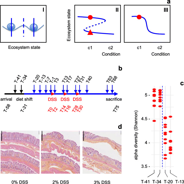
Fig. 1.
Experimental design. a Alternative stable states. Subpanel I, alternative stable states of an ecosystem as beads in a stability landscape. Dashed line, frontier between two basins of attraction. Subpanel II, alternative states (solid lines) can both exist under a range of identical conditions (bi-stable range). Dashed line, see subpanel I. Width and shape of the basins of attraction, and thereby the stability of the alternative states, change with changing conditions, as illustrated by the changing distances between solid lines and the dashed line [14]. When changing conditions push the ecosystem beyond a tipping point (sharp bend in the Z-shape curve), the limit of resilience where the basin of attraction of its present state disappears, it rapidly transits to an alternative state. Subpanel III, steep gradient where for any given condition only one stable state exists. Assuming that the original ecosystem state is represented by the red dot, models II and III both predict a change of ecosystem state when the external conditions change from c1 to c2. When the conditions change back to c1, model II predicts that the system remains in the alternative state (red triangle), while in model III the system returns to its original state. b Timeline of the experiment. Black and blue solid lines, different diets as indicated in the text (diet shift at T-31). Small arrows, fecal sampling time-points. DSS, DSS treatment periods (3 days each). T, time in days relative to start of first DSS treatment (T0). Reception of animals at T-58, sacrifice and distal colon histology at T75. c Reduction of microbiota diversity after diet shift (T-31). Time-points are indicated at the bottom of the figure. Each dot represents one rat. d Induction of low-grade inflammation through DSS treatments. Distal colon histology, 45 days after last DSS treatment. Size bar, 250 μm

