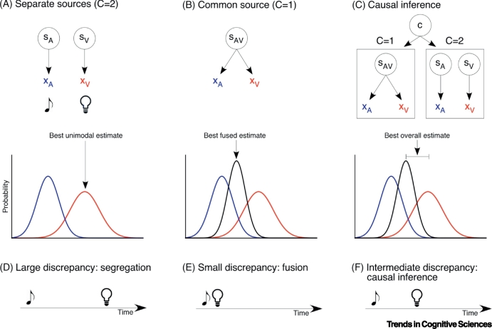
Figure I.

Computational Modelling of Cross-modal Interactions.

(A–C) The first row depicts a schematic representation of different causal structures in the environment. S_A, S_V, and S_AV represent sources of auditory, visual, or cross-modal stimuli, and X_A and X_V indicate the respective sensory representations (e.g., time or location). The bottom row depicts the probability distributions of these sensory representations derived from the Bayesian model. (A) Assuming separate sources (C=2) leads to independent estimates for auditory and visual stimuli, with the optimal value matching the most likely unimodal response. (B) Assuming a common source (C=1) leads to fusion of the two sensory signals. The optimal Bayesian estimate is the combination of both auditory and visual input, each weighted by its relative reliability. (C) In Bayesian Causal Inference, the two different hypotheses about the causal structure (e.g., one or two sources) are combined, each weighted by its inferred probability given the auditory and visual input, known as model averaging. The optimal stimulus estimate is a mixture of the unimodal and fused estimates. (D–F) Schematized temporal relations between two stimuli. (D) When stimuli are presented with large temporal discrepancy, they are typically perceived as independent events and are processed separately. (E) When auditory–visual stimuli are presented with no or little temporal discrepancy, they are typically perceived as originating from the same source and their spatial evidence is integrated (fused). (C) When the temporal discrepancy is intermediate, causal inference can result in partial integration: the perceived timings of the two stimuli are pulled towards each other but do not converge.