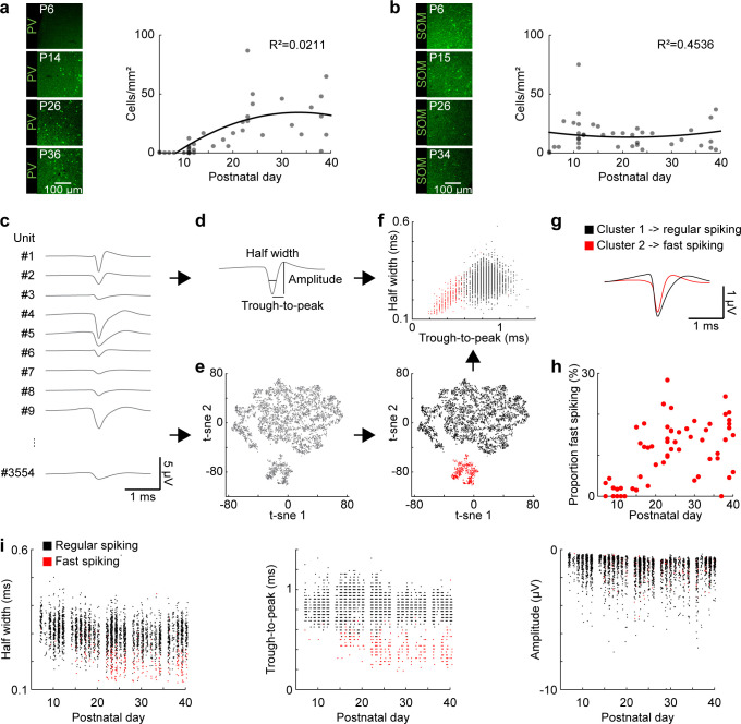
Figure 2. Development of FS interneurons in the mouse mPFC.
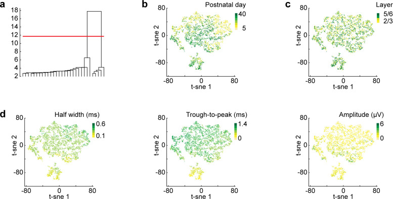
(a) Left, examples of PV immunostaining in the mPFC at different ages. Right, scatter plot displaying the density of PV-immunopositive neurons in the mPFC of P5-40 mice (n = 38 mice). (b) Same as (a) for SOM-immunopositive neurons (n = 39 mice). (c) Example mean waveforms of extracellular recorded single units from P5-40 mice. (d) Schematic showing features classically used to distinguish RS and FS units in adult mice. (e) Left, scatter plot showing the first two components of a t-sne dimensionality reduction on the mean waveforms for all units recorded from P5-40 mice (n = 3554 units from 66 recordings/mice). Right, same as left with the first two clusters obtained by hierarchical clustering labeled in black and red. (f) Scatter plot of half width and trough-to-peak time for cluster 1 (black) and 2 (red). (g) Mean waveform for cluster 1 (black) and 2 (red). (h) Scatter plot showing the proportion of FS units for P5-40 mice. (i) Scatter plots showing classic spike shape features for P5-40 for cluster 1 (RS, black) and 2 (FS, red). (See Supplementary file 1 for a summary of experimental conditions. See Supplementary file 2 for statistics).


