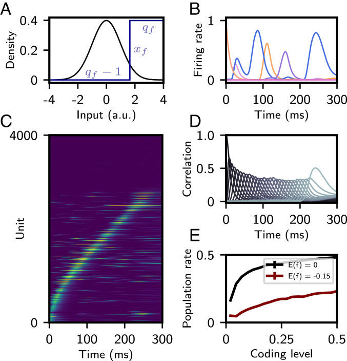
Fig. 4.

Sparse sequences with a nonlinear learning rule. (A) Probability density of Gaussian input pattern $\xi$ (black). Step function $f$ binarizing the input patterns prior to storage in the connectivity matrix (blue) is shown. (B) Firing rate of several representative units as a function of time. (C) Firing rates of 4,000 neurons (out of 40,000) as a function of time, with “silent” neurons shown on top and active neurons on the bottom, sorted by time of peak firing rate. (D) Correlation of network activity with each stored pattern. (E) Average population rate as a function of “coding level” (probability that input pattern is above $x_f$). The average of $\text{f}\left(x\right)$ is maintained by varying $q_f$ with $x_f$. In red, the average of $\text{f}\left(x\right)$ is constrained to $-0.15$, the value in A–D. In black, the average of $\text{f}\left(x\right)$ is fixed to zero. All other parameters are as in A–D. For A–D, parameters of the learning rule were $x_f=1.645$, $x_g=1.645$, $q_f=0.8$, and $q_g=0.95$. $S=1$, $P=30$.