Fig. 2.

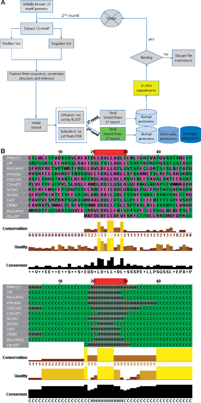
Flowchart of the LDMF tool, and features of the predicted LD motif sequences. (A) Our learning process contains three iterations. The first iteration was by training a support vector machine (SVM) model based on the 18 known LD motifs as the positive set and randomly drawn sequences as the negative one. Sequence, secondary structure and AAindex features of these sets were used to build an initial model. This model was expected to have poor prediction performance because the randomly drawn negative sequences are expected to be easily differentiable from the positive ones. We then applied this initial model to identify putative LD motifs in close orthologs of our six positive-set proteins, using standard protein–protein unidirectional BLAST (blastp) (Altschul et al., 1997) (see Supplementary Material for details). This step resulted in additional 40 LD motif sequences that we manually checked and added to the positive set. The initial model was then applied to the protein data bank (PDB) to find sequences that satisfy some of the key features, but not all of them. These sequences are similar to the true motifs in some aspects and thus provide a much more difficult negative set for the second iteration of training. These training sets were used to build the ‘final’ first round model, with which we scanned the human proteome (20 159 sequences). All predicted novel LD motifs were synthesized as peptides and used in in vitro binding experiments. Those sequences that showed binding were included in the positive set of the final iteration of training. The final model of the second round was used to predict LD motifs in various proteomes. (B) The ten amino acids constituting the LD motif core are highlighted inside the red box. The twenty up- and down-stream residues of the flanking regions are shown. Top: amino acid sequences. Bottom: secondary structure. This figure was generated by Jalview (Waterhouse et al., 2009)