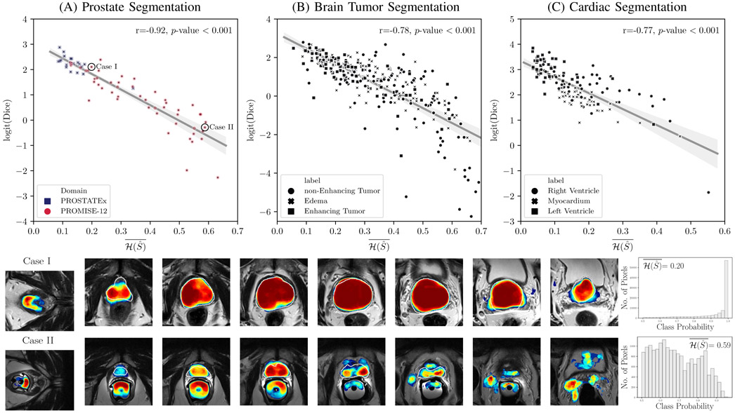
Fig. 3.
Segment-level predictive uncertainty estimation: Top row: Scatter plots and linear regression between Dice coefficient and average of entropy over the predicted segment . For each of the regression plots, Pearson’s correlation coefficient (r) and 2-tailed p-value for testing non-correlation are provided. Dice coefficients are logit transformed before plotting and regression analysis. For the majority of the cases in all three segmentation tasks, the average entropy correlates well with Dice coefficient, meaning that it can be used as a reliable metric for predicting the segmentation quality of the predictions at test-time. Higher entropy means less confidence in predictions and more inaccurate classifications leading to poorer Dice coefficients. However, in all three tasks there are few cases that can be considered outliers. (A) For prostate segmentation, samples are marked by their domain: PROSTATEx (source domain), and the multi-device multi-institutional PROMISE12 dataset (target domain). As expected, on average, the source domain performs much better than the target domain, meaning that average entropy can be used to flag out-of-distribution samples. The two bottom rows correspond to two of the cases from the PROMISE12 dataset are marked in (A): Case I and Case II; These show the prostate T2-weighted MRI at different locations of the same patient with overlaid calibrated class probabilities (confidences) and histograms depicting distribution of probabilities over the segmented regions. The white boundary overlay on prostate denotes the ground truth. The wider probability distribution in Case II associates with a higher average entropy which correlates with a lower Dice score. Case-I was imaged with phased-array coil (same as the images that was used for training the models), while Case II was imaged with endorectal coil (out-of-distribution case in terms of imaging parameters). The samples in scatter plots in (B) and (C) are marked by their associated foreground segments. The color bar for the class probability values is given in Figure 1. Qualitative examples for brain and heart applications and scatter plots for models trained with cross-entropy are given in Figures 7 and 8 of the Supplementary Material, respectively.

