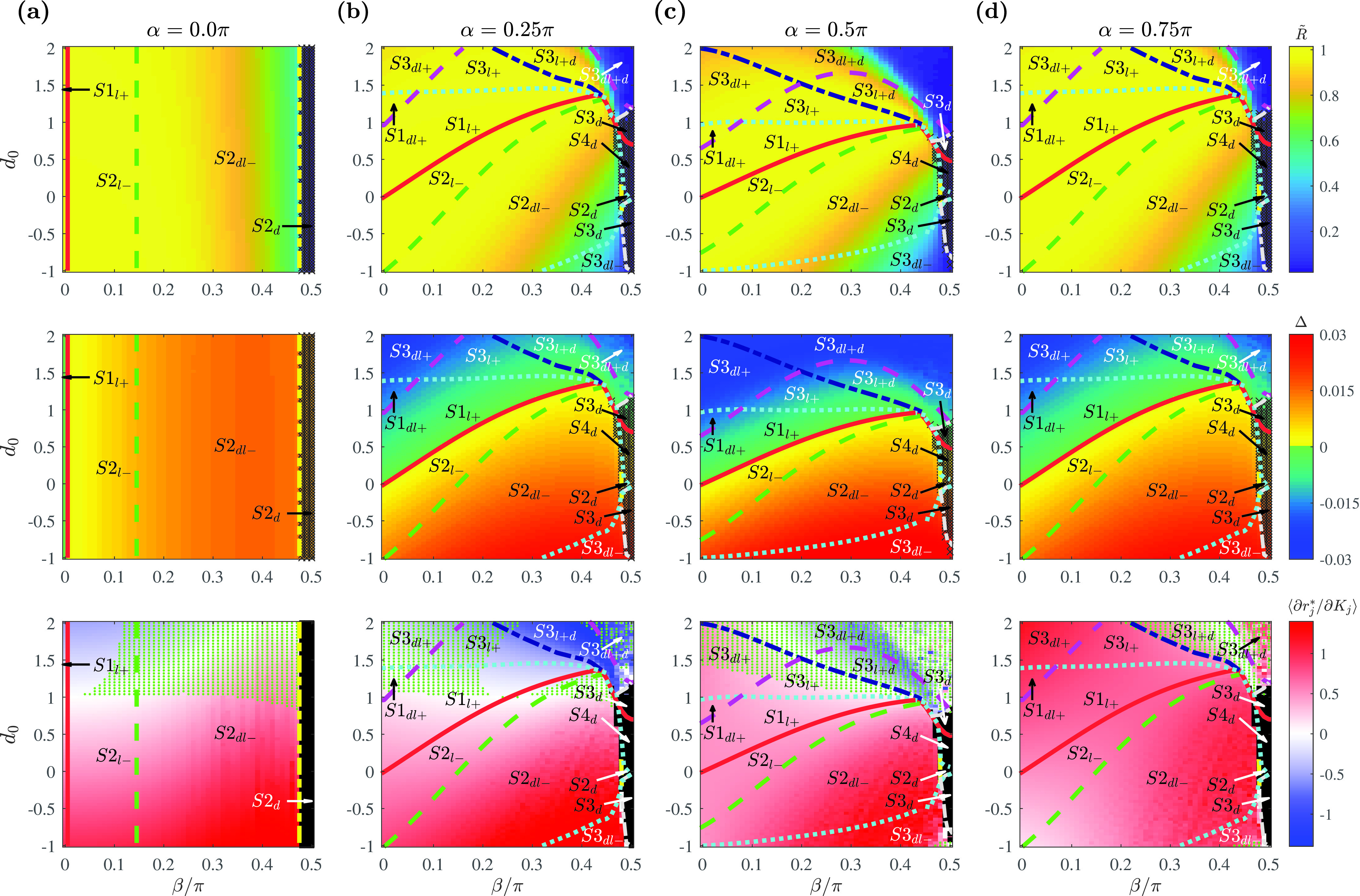
FIG. 3.

Phase diagrams with the Gaussian coupling strength distribution as a function of $\alpha$, $\beta$, and $d_0$ determining the shape of the coupling function. Representative fixed values of $\alpha$ are chosen at (a) $\alpha =0$ where $\sin \alpha =0,\cos \alpha =1$, (b) $\alpha =0.25\pi$ where $\sin \alpha >0,\cos \alpha >0$, (c) $\alpha =0.5\pi$ where $\sin \alpha =1,\cos \alpha =0$, and (d) $\alpha =0.75\pi$ where $\sin \alpha <0,\cos \alpha >0$. Phase diagrams with order parameter $\tilde{R}$ (first row), phase spread $\mathrm{\Delta }=\omega -\mathrm{\Omega }$ (second row), and the slope of the amplitude curve $(K_j,{r_j}^{\ast })$ calculated as the average value of $\frac{\mathrm{\partial }{r}_j^{\ast }}{\mathrm{\partial }{K}_j}$ among the locked oscillators (third row). Regions with fully drifting population are marked in black. For the amplitude slope, the parameter space in which the inflection point exists in the $(K_j,{r_j}^{\ast })$ curve (from a positive to negative slope) is additionally marked with green dots. The boundaries are determined numerically from the model equation (1) for a Gaussian distribution with $(K_{\text{mean}},{\sigma }_K,K_{\text{min}},K_{\text{max}})=(20.2,4.36,7.85,34.4)\times {10}^{-3}$. The bounding curves are obtained for $\mathrm{\Delta }=0$ (solid red), $\tilde{R}=|d_0\sin \alpha |⟨{r_j}^{\ast }⟩$ (dotted cyan), $\frac{\mathrm{\Delta }{r_{\text{min}}}^{\ast }}{\tilde{R}-|d_0\sin \alpha |{r_{\text{min}}}^{\ast }}=K_{min}$ (dashed green), $\frac{|\mathrm{\Delta }|{r_{\text{min}}}^{\ast }}{\tilde{R}+|d_0\sin \alpha |{r_{\text{min}}}^{\ast }}=K_{min}$ (long dashed magenta), $\frac{|\mathrm{\Delta }|{r_{\text{max}}}^{\ast }}{|d_0\sin \alpha |{r_{\text{max}}}^{\ast }-\tilde{R}}=K_{max}$ (dashed–dotted navy), $\frac{\mathrm{\Delta }{r_{\text{max}}}^{\ast }}{\tilde{R}-|d_0\sin \alpha |{r_{\text{max}}}^{\ast }}=K_{max}$ (dashed–dotted yellow), $\frac{|\mathrm{\Delta }|\sqrt{\lambda }}{|d_0\sin \alpha |\sqrt{\lambda }-\tilde{R}}=K_{min}$ (dashed–dotted gray, $d_0\ge 0$), and $\frac{\mathrm{\Delta }\sqrt{\lambda }}{\tilde{R}+|d_0\sin \alpha |\sqrt{\lambda }}=K_{max}$ (dashed–dotted gray, $d_0<0$). Simulation parameters: $\lambda =1$, $\omega =\pi$, $S=1$, $N=1000$.