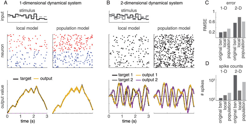
Fig 6. Simulations of the local and population frameworks implementing a 1D and 2D dynamical system.

(A) The target was a 1-dimensional integrator: $\dot{x}\left(t\right)=c\left(t\right)$. Left side shows spikes and outputs from local Poisson model, while right side shows spikes and outputs for population Poisson model. As in previous figures, red dots indicate spikes from neurons with positive output weights, blue dots indicate spikes from neurons with negative weights. (B) The target was a 2-dimensional oscillator ${\dot{x}}_1\left(t\right)=-x_1\left(t\right)-10x_2\left(t\right)+c\left(t\right);x_2\left(t\right)=10x_1\left(t\right)-x_2\left(t\right)+c\left(t\right)$. For the population model, the time window for computing expected spike count was κ = 5ms (50 time bins). Weights were randomized to be positive or negative in either dimension, such that neurons are no longer divided into strictly positive- or negative-weight groups. (C) Accuracy (measured by root-mean-squared error) of the two models for 1D and 2D systems. (D) Number of spikes emitted by each model during simulations (log scale).