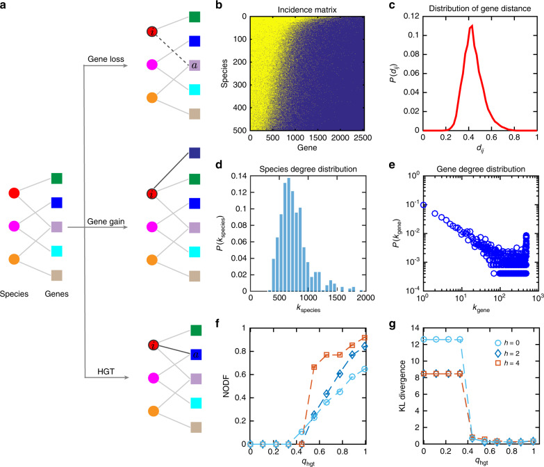
Fig. 4. A simple genome evolution model can generate GCNs that capture key topological features of the real GCN.

a Schematic diagram of the genome evolution model. At each time step t, the genome of a species i (shown in red) randomly chosen with probability proportional to $k_i^h$ will be updated based on one of the following three events: gene loss, gene gain, and horizontal gene transfer (HGT), with corresponding rates q_gl, q_gg, q_HGT, respectively. Note that the parameter h ≥ 0 representing the selection pressure, and h = 0 corresponds to the case of neutral model. The three rates naturally satisfy q_gl + q_gg + q_HGT = 1. During HGT, a gene a from a randomly chosen donor species is randomly selected and then transferred to the genome of species i. During gene loss, a gene a in the genome of species i is randomly selected and then removed. During gene gain, a new gene is added to the genome of species i. The initial GCN is a random bipartite graph that consists of 500 species and 200 genes with connection probability 0.8. The total number of evolution time steps is 5 × 10⁵. b–e The incident matrix of the final GCN (with nestedness value NODF = 0.703), functional distance, species degree and gene degree distributions with h = 2, q_HGT = 0.795, q_gg = 0.005, and q_gl = 0.2 (See Supplementary Figs. 12, 13 for those topological features with other model parameters). f The nestedness (quantified by NODF) of the final GCN calculated as a function of HGT rate with different selection pressure h = 0,2,4. g The Kullback–Leibler (KL) divergence between the normalized gene degree distribution $P\left({\tilde{k}}_{\mathrm{gene}}\right)$ of real GCN and that of the simulated GCNs calculated with different selection pressures and HGT rates as shown in f. Here the normalized gene degree ${\tilde{k}}_{\mathrm{gene}}\equiv k_{\mathrm{gene}}/k_{\mathrm{gene}}^{\max }$.