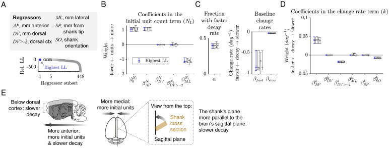
Figure 5. The initial unit count depends on the AP and ML positions, and the rate of decay depends on the AP position, whether an electrode is in dorsal cortex, and the shank orientation.

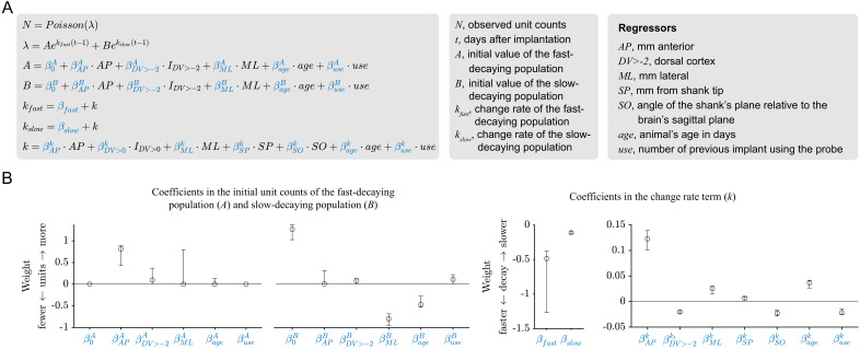
(A) A sum-of-exponentials regression (SoER) model was fit to the number of units recorded from each electrode in each session (N = 57,586 recordings) to infer the relationship between experimental factors and unit loss over time. Continuous regressors AP, DV, ML, SP, and SO indicate an electrode’s position in millimeters anterior, dorsal, lateral, and from the shank tip, and the orientation (in degrees) between the shank’s plane from the brain’s sagittal plane, respectively. Categorical regressors DV>-2 indicate whether an electrode is in the dorsal cortex. Model variants with different subsets of regressors were ordered by relative out-of-sample log-likelihood (LL). The five subsets with the highest LL are shown in subsequent panels. (B) Coefficients in the equation term indicating the initial unit count (N₁) from the five regressors subsets with the highest LL. Initial unit count consistently depends on AP and ML (orange), which are included and significantly nonzero in the top five models. Error bars indicate 95% bootstrap confidence intervals. The range of all regressors is normalized to be [0,1] to facilitate comparison. The original range of the regressors were AP [−7.40, 4.00], DV [−9.78,–0.01], ML [0.29, 5.59], SP [0.02, 7.68], SO [0, 90]. (C) About 40% (α) of the units disappeared rapidly with a baseline change rate of −0.87 (k_fast), and the remaining disappeared more slowly with a baseline change rate of −0.03 (k_slow). (D) Change rates depended consistently on the regressors AP, DV>-2 (whether the unit was in dorsal cortex), and SO (angle between the shank’s plane and the brain’s sagittal plane), which are included and have a significantly nonzero coefficient in the top five models. (E) A graphical summary of the modeling results.

Figure 5—figure supplement 1. The results of the sum-of-exponentials regression (SoER) model are corroborated by the results of an elaborated SoER model.

(A) Two additional regressors (the animal’s age and the number of times a probe was previously used for chronic implantation) are added to the elaborated model. The initial unit counts of the fast- and slow-decaying population in the basic model depend on separate linear combinations of the regressors (A and B), whereas in the basic model they depended on a single linear combination of the regressors (N) and a scaling parameter (α). The variable Y is a vector of observed unit count on each electrode pooled across all recordings and is assumed to follow a Poisson distribution, and the λ parameter of the Poisson distribution is a sum of two exponentials. The parameter t is the number of days after implantation, A is the initial unit count of the fast-decaying population, and B is the initial unit count of the slow-decaying population. The parameters k_fast and k_slow are the exponential change rates of the fast- and slow-decaying populations, respectively. Note that these two parameters differ by a constant offset (β^k_fast – β^k_slow) and depend on the same linear combination of the regressors (k). (B) Maximum-likelihood estimates of the model parameters. The model was fit using L1 (LASSO) regularization to sparify coefficient estimates. Error bars indicate bootstrapped 95% confidence interval. Similar to the basic model, the initial unit counts depended on the regressors AP and ML and the changes rates depended on the regressors AP, DV>-2, and SO.