Figure 5.

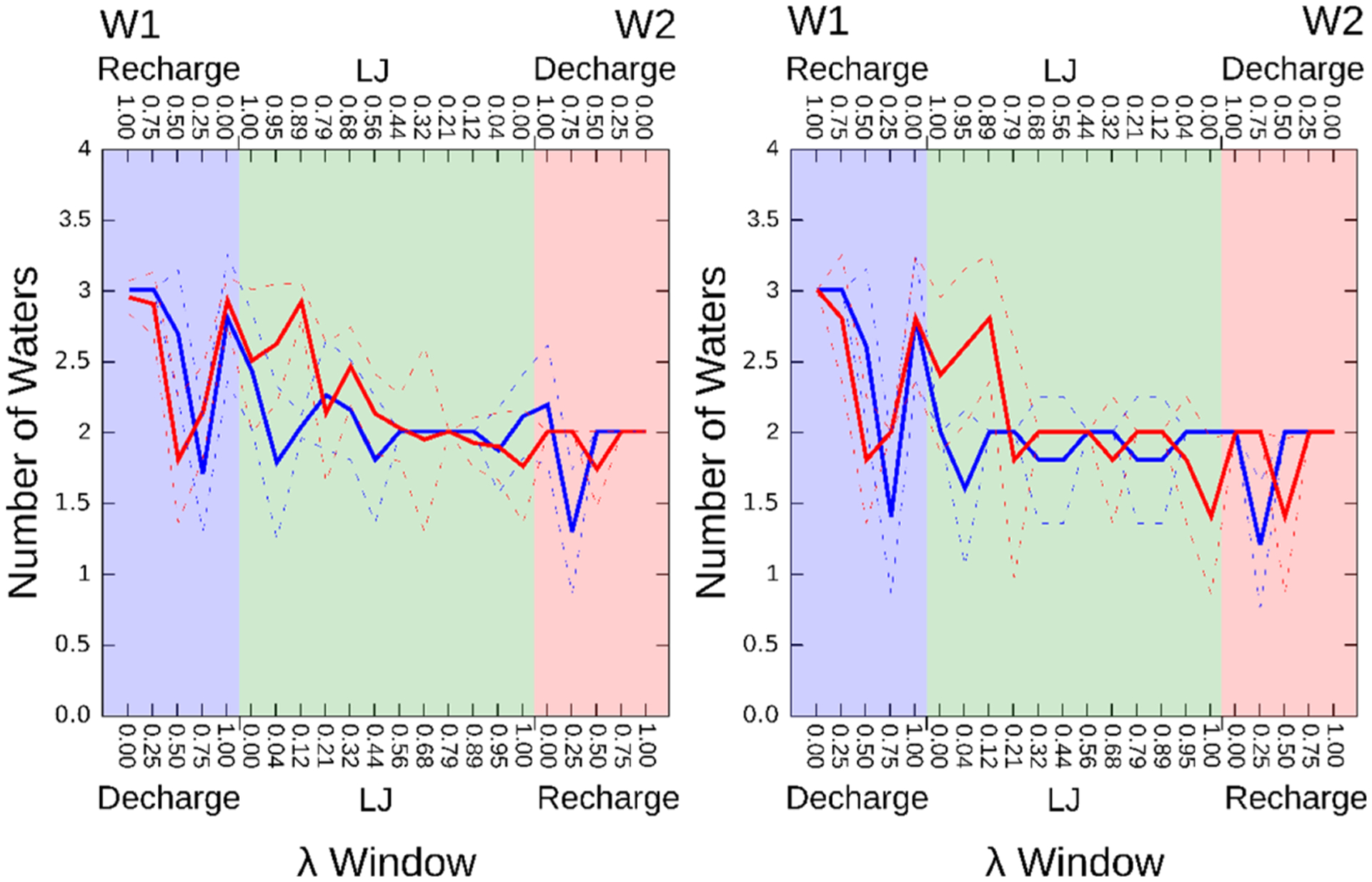
Computed mean water occupancies for each λ window in the W1–W2 perturbation. Blue: Perturbation W1 → W2 with the λ windows labeled at the lower X-axis. Red: Reverse perturbation, W2 → W1, with λ windows in reverse order as labeled at the upper X-axis. Dashed lines: show ranges defined by the standard deviations over the five repetitions. Left: Number of buried water molecules after the water equilibration step shared by methods 1 and 2 (see Figure 2), averaged over the five replicates. Right: Time- and replica-averaged number of buried water molecules for each λ window in the five TI production runs of method 1.