
Figure 5.
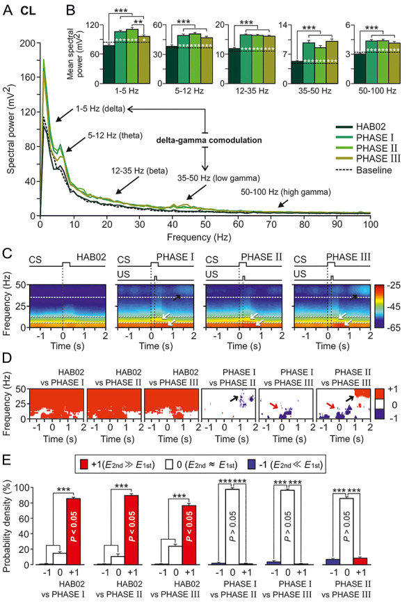
Spectral analyses of LFPs recorded in the CL during classical eyeblink conditioning. LFPs were recorded during habituation and conditioning phases from four rabbits. (A) Mean power spectra of LFPs recorded in the CL for 120 3.5 s frames (between 1.5 s before and 2 s after CS presentation) for four of the conditions (HAB02, phase I, phase II, and phase III) and for 3.5 s baseline frames (taken from HAB02 sessions but including no stimulus). The black arrows indicate the spectral rangescorresponding to delta (1–5 Hz), theta (5–12 Hz), beta (12–35 Hz), and low- (35–50 Hz) and high- (50–100) gamma bands. Although the fundamental contribution to CL power spectrum was determined by delta and theta frequency bands, prominent (well-differentiated) power peaks appeared in delta and low gamma bands during phases I and III. Therefore, the resulting delta–gamma comodulation is also indicated. (B) Histograms of mean spectral powers for all the defined frequency bands. Note that the start of conditioning phases significantly increased the spectral powers in the five frequency bands (Tukey–Kramer multiple comparison test: HAB02 and Baseline vs. phases I, II, and III; ***P < 0.001). Also note that baseline values (dotted black line) were very similar to those collected during the presentation of the unpaired CS (HAB02). (C) Time–frequency representations (spectrograms; NT × K = 600 tapered Fourier transforms) corresponding to data from HAB02 and conditioning phases I, II, and III illustrated in A and B. Note that maximum spectral powers (see the color calibration bar at the right) for delta and theta occurred during and shortly after CS/US presentations, in the three conditioning phases (white arrows), but maxima for low gamma appeared 1 s after the CS/US, during phases I and III (black arrows). (D) Multiple comparisons between the different spectrograms and their corresponding probabilistic maps according to the jackknifed variance criterion. Red (inference type +1; power in first spectrogram ≫ power in second spectrogram) and blue (inference type −1; power in first spectrogram ≪ power in second spectrogram) indicate significant statistical differences (P < 0.05; jackknifed estimates of the variance), and white (inference type 0; power in first spectrogram ≈ power in second spectrogram) indicates no significant differences (P > 0.05). Black arrows indicate that the spectral powers in the low-gamma frequency band were higher in phases I and (especially) III when comparing with phase II; that increment occurred at the end (range between 1 and 2 s after the CS/US presentation) of the analyzed epoch. Red arrows show how, in contrast, spectral powers in low frequencies were higher in phases I and (especially) II when comparing with phase III during and slightly after the CS/US presentation. (E) Histograms of mean probability densities. Here, it is very evident (***P < 0.001, Tukey–Kramer test) that there are statistically significant differences (P < 0.05, red bars) between the habituation (HAB02) and the conditioning (I, II, and III) phases in practically the whole time–frequency range. Although they present some specific significant differences in delta, theta, and low gamma bands, the three conditioning sessions are not statistically different overall (P > 0.05, white bars).