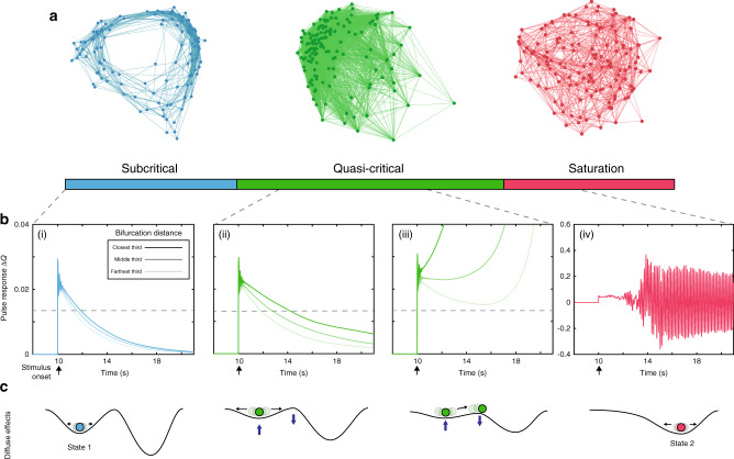
Fig. 3. Properties of quasi-critical states.
a Average regional correlations within each zone shown as a force-directed graph. b For a given χ, each node was stimulated with an excitatory rectangular pulse (amplitude = 1 mV; width = 10 ms) at t = 10 s. The target nodes activity was then compared to simulated activity in the absence of the pulse using the same noise sequence in order to quantify the perturbation induced. The pulse results are sorted based on their mean distance to bifurcation in the preceding 8 time points. For visualization purposes we then average the activity within the closest, middle, and farthest thirds based on this sorted distance, and low-pass filtered with a passband frequency of 0.001 Hz. (i) χ = 1.15 × 10⁻⁴ (ii) χ = 1.21 × 10⁻⁴ (iii) χ = 1.25 × 10⁻⁴ (iv) χ = 1.3 × 10⁻⁴ mV s; Note the vertical axis on (iv) differs from (i)–(iii). c Qualitative effect of increasing diffuse coupling on the attractor landscape: in the subcritical zone, the system was enslaved to the lower attractor; increasing χ into the quasi-critical zone had the effect of flattening the attractor landscape, allowing noise-driven excursions to transition nodes across their local bifurcation point; at high values of χ, the system became enslaved to the higher attractor.

