Modeling dynamic radial contrast enhanced MRI with linear time invariant systems for motion correction in quantitative assessment of kidney function

Abstract

Early identification of kidney function deterioration is essential to determine which newborn patients with congenital kidney disease should be considered for surgical intervention as opposed to observation. Kidney function can be measured by fitting a tracer kinetic (TK) model onto a series of Dynamic Contrast Enhanced (DCE) MR images and estimating the filtration rate parameter from the model. Unfortunately, breathing and large bulk motion events due to patient movement in the scanner create outliers and misalignments that introduce large errors in the TK model parameter estimates even when using a motion-robust dynamic radial VIBE sequence for DCE-MR imaging. The misalignments between the series of volumes are difficult to correct using standard registration due to 1) the large differences in geometry and contrast between volumes of the dynamic sequence and 2) the requirement of fast dynamic imaging to achieve high temporal resolution and motion deteriorates image quality. These difficulties reduce the accuracy and stability of registration over the dynamic sequence. An alternative registration approach is to generate noise and motion free templates of the original data from the TK model and use them to register each volume to its contrast-matched template. However, the TK models used to characterize DCE-MRI are tissue specific, non-linear and sensitive to the same motion and sampling artifacts that hinder registration in the first place. Hence, these can only be applied to register accurately pre-segmented regions of interest, such as kidneys, and might converge to local minima under the presence of large artifacts. Here we introduce a novel linear time invariant (LTI) model to characterize DCE-MR data for different tissue types within a volume. We approximate the LTI model as a sparse sum of first order LTI functions to introduce robustness to motion and sampling artifacts. Hence, this model is well suited for registration of the entire field of view of DCE-MR data with artifacts and outliers. We incorporate this LTI model into a registration framework and evaluate it on both synthetic data and data from 20 children. For each subject, we reconstructed the sequence of DCE-MR images, detected corrupted volumes acquired during motion, aligned the sequence of volumes and recovered the corrupted volumes using the LTI model. The results show that our approach correctly aligned the volumes, provided the most stable registration in time and improved the tracer kinetic model fit.

1. Introduction

Accurate assessment of kidney function and anatomy in newborns and children with hydronephrosis is clinically important. Patients require surgical intervention as opposed to observation when there is clear evidence of obstruction of the urinary tract and renal function deterioration. For these conditions, as well as other conditions affecting kidney function in both children and adults, timely determination of which patients have renal dyfunction or deterioration is important since delays in intervention can lead to potential lifelong complications and chronic renal insufficiency Chevalier (1995); Chevalier et al. (2010). In current clinical practice, kidney function, i.e. glomerular filtration rate (GFR) is estimated based on serum creatinine and drainage times and differential renal function is estimated based on nuclear renography Grattan-Smith et al. (2008); Michaely et al. (2008); Chandarana et al. (2014). However, serum creatinine is not sensitive to early decline in function and nuclear renography is invasive, has low spatial and contrast resolution, does not provide anatomic information and exposes the patient to ionizing radiation, which makes it unsuitable as a routine monitoring test, especially for children.

Dynamic Contrast Enhanced (DCE) MRI is an imaging technique with great potential since it provides both a detailed anatomical evaluation of kidneys and qualitative and quantitative information about kidney function at the same time Grattan-Smith et al. (2008). Another advantage is that, unlike nuclear renogram techniques, MRI does not expose patients to ionizing radiation and is superior in terms of spatial resolution, which enables differentiated evaluation of kidney compartments, including cortex, calyces and medulla as well as renal arteries and urinary tract.

DCE-MRI consists of acquisition of a continuous sequence of MRI volumes during which a contrast agent is injected into the bloodstream and filtered through the kidneys. This dynamic series of images allow radiologists to qualitatively evaluate the temporal evolution of the contrast agent through the kidney compartments, where a delay in contrast reaching the calyces may indicate obstruction in the urinary tract and may require surgical correction. At the same time, quantitative evaluation with the appropriate tracer kinetic models can provide important markers of kidney function including the perfusion rate in the cortex and the filtration rate in the kidneys. Moreover, it is possible to quantitatively evaluate the relative function of the right and left kidneys, i.e. differential renal function, the absolute function of each kidney, and to generate a voxelwise functional map for assessment of regional function in duplex kidneys.

We recently showed that DCE-MRI acquisition with a dynamic radial VIBE sequence is both robust to respiratory motion and can attain high temporal and spatial resolution (3s, 1.25 × 1.25 × 3 mm) for accurate estimation of AIF peak Block et al. (2014); Kurugol et al. (2017a, 2018); Coll-Font et al. (2019c,b); Kurugol et al. (2019, 2020). Specifically, we acquired k-space data with a golden angle stack-of-stars sampling scheme and reconstruct images from undersampled data with high spatio-temporal resolution using a compressed-sensing method with temporal regularization to minimize the undersampling artifacts Feng et al. (2014); Chandarana et al. (2015); Kurugol et al. (2019); Coll-Font et al. (2019b); Kurugol et al. (2020).

Despite using a motion-compensated sequence, heavy breathing or bulk motion of the patient due to discomfort and the extended length of the scan (∼ 6min), can still affect the quality of the imaging. This is particularly problematic for infants imaged without sedation Kurugol et al. (2019), using feed and wrap imaging technique, who often move their bodies during their scan. These bulk motion events deteriorate the quality of the images, introduce blurring, signal dropout and cause misalignment between volumes within the dynamic series. As a result, these artifacts limit the diagnostic quality of the images and dramatically reduce the accuracy of quantitative evaluation of kidney function. Moreover, since DCE-MRI requires injection of contrast agent during acquisition, the scans cannot be easily repeated when the subject moves and consequently the imaging provides incomplete information.

In order to correct for the misalignment created by bulk motion events, it is necessary to register the DCE-MR sequence. However, contrast agent intake in the body generates large changes in both the signal intensity and the geometry of the volumes over time, and therefore volumes at different time points look quite different from each other. This limitation complicates the registration between image pairs, especially if they are acquired at distant time points, and particularly for those acquired before injection of contrast. Moreover, streaking artifacts and low SNR due to undersampled acquisition (for high temporal resolution) reduce the image quality and make the ill-posed task of registration even more challenging and an outstanding problem in DCE-MRI.

There have been extensive efforts in the research community to address the challenge of registration in DCE-MRI. However, each technique has its limitations and there is no agreement to which registration technique is best suited for this problem Zöllner et al. (2019). Some researchers registered each volume in the sequence against a reference volume and used registration metrics that are robust to contrast variations. Typical metrics are cross-correlation, normalized gradients Merrem et al. (2013); Hodneland et al. (2014b), mutual information and normalized mutual information Hodneland et al. (2014a); Positano et al. (2013); Fei et al. (2005); Melbourne et al. (2011) or sum-of-squares difference after equalization of the contrast between images Wright et al. (2014). Since these approaches register individual volumes to a single reference, they can compensate for rapid changes in position of the subject –i.e. bulk motion events. However, the motion and undersampling artifacts in the images introduce registration errors to each volume and, consequently, volume-to-volume variability in the alignment of the sequence. On the other hand, more recent work has focused on groupwise metrics to jointly register an entire sequence of volumes. These metrics often minimize the variance or discrepancy of the registered volumes over time with low rank approximations Melbourne et al. (2007); Hamy et al. (2014); Huizinga et al. (2016); Johansson et al. (2016). These reduce the volume-to-volume variability of the registration, but might not capture the sudden changes in position of the subject. An alternative approach to balance stability and rapid motion consists of registering individual volumes using the tracer kinetic (TK) model Adluru et al. (2006); Buonaccorsi et al. (2005, 2007) or the signal decay model Kurugol et al. (2017b) itself. This approach allows to compensate for rapid bulk motion –since each volume is registered independently– while introducing robustness to artifacts with the noise free templates generated with the signal model. Unfortunately, the TK models are specific to organs of interest (e.g. kidneys), therefore, they cannot fit well to the neighboring tissue types Buonaccorsi et al. (2006) and their fitting is sensitive to motion and undersampling artifacts in the data. Consequently, TK model-based registration cannot be applied to the entire field of view. It requires accurate segmentation of the region of interest, such as kidneys, leaving other tissue in the image, and aorta, which is important for tracer kinetic model fitting, misaligned. This reduces the accuracy of the TK model fitting in the kidneys.

To be able to characterize the entire field of view and overcome introduce a Linear Time Invariant (LTI) model based motion correction (LiMo-MoCo) algorithm. Our approach, depicted in Fig. 1, uses and LTI model to characterize the signal intensity for all tissues – including aorta, kidneys as well as the other neighboring tissues– and generate a template with matched contrast levels to which the original volumes can be registered. Unlike previous work using LTI models for DCE-MRI Caldeira and Sanches (2008), we approximate the LTI model as a sparse sum of first order LTI functions, which 1) avoids convergence to local minima and 2) reduces the sensitivity to outliers. This approach ensures that the reference image for registration is a noise-free template with similar appearance to the moving image, thus simplifying the task of registration. This paper extends our model-driven motion compensation framework for renal dynamic radial DCE-MRI, originally presented at the MICCAI 2019 conference. We provide a more detailed description of the model, and an extensive additional set of simulated experiments Coll-Font et al. (2019a) and analysis. We also extended the dataset composed of patient data to more extensively analyze the quality of the resultant images, the estimated time-intensity curves and the quantitative parameters after LTI model based motion compensation in comparison to previous approaches.

Fig. 1.

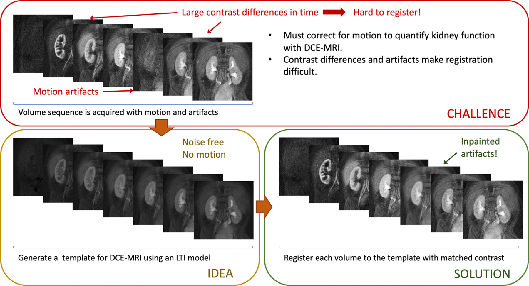
Visual abstract depicting the basic principles of this work. The DCE-MRI data acquired from the patients is misaligned due to motion and corrupted when acquired during motion events. Aligning the dynamic sequence of volumes is challenging due to differences in contrast between volumes and the presence of artifacts lowering the quality of each image. Our approach fits an LTI model to the data and reconstructs a noise and motion free sequence of dynamic template volumes. The method then registers every volume to its template with matched contrast and interpolates the outlier volumes corrupted by motion.

2. Methods

2.1. LTI model for tissue contrast enhancement

Most tracer kinetic models characterize the signal intensity in DCE-MRI, s(t), as the convolution of the arterial input function (i.e. the contrast agent introduced through the arteries), a(t), with a system response, h(t), that describes the filtration of the contrast through the kidneys:

$$s\left(t\right)=h\left(t\right)\ast a\left(t\right).$$ (1)

Typically, these tracer kinetic models describe the unknown tissue response h(t) as the composition of multiple leaky compartments through which the tracer flows Khalifa et al. (2014); Ingrisch and Sourbron (2013). These multi-compartment models are often tailored to a specific type of tissue, and estimating their parameters requires solving a non-linear least-squares optimization problem. Hence, these are not adequate to characterize the signal intensity in an entire DCE-MRI volume series with noisy measurements and motion Buonaccorsi et al. (2006).

To overcome these limitations, we introduced an LTI model to describe the tissue response h(t). Specifically, we approximate the system response as the weighted sum of first-order, strictly-proper LTI transfer functions $g_{p_k}\left(\text{t}\right)$ with weights c_k and poles p_k contained within the section of the unit disk D_ρ.

$$h\left(t\right)=\sum _{p_k\in D_{\rho }}{c}_k{g}_{p_k}\left(t\right)$$ (2)

The advantages of characterizing the DCE-MRI data with this model are threefold. First, the LTI model is flexible enough to characterize a broad set of impulse responses and, hence, tissue types present in an acquired volume. Second, this model is linear with respect to its unknowns –i.e. the weights c_k – and can be solved as a convex optimization problem. Third, the model can be regularized by restricting the poles of the transfer functions $g_{p_k}$ to those in the low frequency disk D_ρ (with normalized frequency ρ < 0.014), and the weights c_k can be estimated using sparsity priors. All these advantages make the resulting model well suited to characterize DCE-MRI data under realistic noise and motion.

To learn the tissue response h(t), it is necessary to solve a convex optimization problem with respect to the unknown weights c_k. Moreover, in order to enforce sparsity, the objective function should find the minimum number of c_k > 0 such that the difference between s(t) and h(t) ∗ a(t) is minimized. This is an NP-hard problem over a infinite dimensional space, hence, it requires to be relaxed in order to be solved. To that objective, we use the randomized system identification method by Yilmaz et. al. Yilmaz et al. (2018). This method solves a convex relaxation of the original l₀ norm minimization problem where the regularization is done through an l₁ norm on the weigths c_k and regularization parameter τ (see Eq. 3):

$$\begin{gathered} \underset{c_k}{\text{min}}\sum _t{\left[s\left(t\right)-\sum _{p_k\in D_{\rho }}{c}_{k}g\left(p_k\right)\left(t\right)\right]}^2 \\ st.\sum _k\left|c_k\right|\le \tau \end{gathered}$$ (3)

We then solve (Eq. 3) with a randomized version of the Frank-Wolfe algorithm Jaggi (2013) described in Algorithm 1. The algorithm follows the basic structure of standard Frank-Wolfe, although here, we randomly select the elements of the atomic set at every iteration. In short, at every iteration ‘i’, the algorithm selects N random poles p_k ∈ D_ρ, computes their corresponding impulse responses ${\left\{g\left(p_k\right)\left(t\right)\right\}}_{n=0}^{N-1}$, and picks the one most aligned with the descent direction. Then, it updates the coefficients c_k such that $f\left(h^{i+1}\right)={\sum }_t{\left[h^{i+1}\left(t\right)\ast a\left(t\right)-s\left(t\right)\right]}^2$ is minimized with $h^{i+1}\left(t\right)=h^i\left(t\right)+c_{k}g\left(p_k\right)\left(t\right)$.

$$\overline{\underset{\_}{\begin{array}{l}\mathbf{\text{Algorithm}}\hspace{0.17em}\mathbf{1}\hspace{0.17em}\hspace{0.17em}\text{LTI}\hspace{0.17em}\text{model}\hspace{0.17em}\text{fit}.\\ \overline{\begin{array}{l}1:\hspace{0.17em}\hspace{0.17em}\mathbf{\text{procedure}}\hspace{0.17em}\text{LTIFIT}\left(a\left(t\right),s\left(t\right)\right)\\ 2:\hspace{0.17em}\hspace{0.17em}\hspace{0.17em}\hspace{0.17em}\hspace{0.17em}\hspace{0.17em}\hspace{0.17em}{x}_0\leftarrow g_{p_0}\left(t\right)\\ 3:\hspace{0.17em}\hspace{0.17em}\hspace{0.17em}\hspace{0.17em}\hspace{0.17em}\hspace{0.17em}\hspace{0.17em}\mathbf{\text{for}}\hspace{0.17em}k=1,2,\dots ,K_{\text{max}}\hspace{0.17em}\mathbf{\text{do}}\\ 4:\hspace{0.17em}\hspace{0.17em}\hspace{0.17em}\hspace{0.17em}\hspace{0.17em}\hspace{0.17em}\hspace{0.17em}\hspace{0.17em}\hspace{0.17em}\hspace{0.17em}\hspace{0.17em}\hspace{0.17em}\text{Select}\hspace{0.17em}N\hspace{0.17em}\text{poles}\hspace{0.17em}\text{randomly}\hspace{0.17em}\text{distributed}\hspace{0.17em}\text{over}\hspace{0.17em}{g}_{p_n}\left(t\right)\in {\mathcal{D}}_{\rho }\end{array}}\\ 5:\hspace{0.17em}\hspace{0.17em}\hspace{0.17em}\hspace{0.17em}\hspace{0.17em}\hspace{0.17em}\hspace{0.17em}\hspace{0.17em}\hspace{0.17em}\hspace{0.17em}\hspace{0.17em}\hspace{0.17em}{g}_{p_k}\left(t\right)\leftarrow argmi{n}_{p_n}<\nabla f\left(x_k\right),g_{p_n}\ast a\left(t\right)>\\ 6:\hspace{0.17em}\hspace{0.17em}\hspace{0.17em}\hspace{0.17em}\hspace{0.17em}\hspace{0.17em}\hspace{0.17em}\hspace{0.17em}\hspace{0.17em}\hspace{0.17em}\hspace{0.17em}\hspace{0.17em}{\alpha }_k\leftarrow argmi{n}_{\alpha =\left[0,1\right]}f\left(x_k+\alpha \left[\tau g_{p_k}\left(t\right)\ast a\left(t\right)-x_k\right]\right)\\ 7:\hspace{0.17em}\hspace{0.17em}\hspace{0.17em}\hspace{0.17em}\hspace{0.17em}\hspace{0.17em}\hspace{0.17em}\hspace{0.17em}\hspace{0.17em}\hspace{0.17em}\hspace{0.17em}\hspace{0.17em}{x}_k\leftarrow x_k+\alpha \left[\tau g_{p_k}\left(t\right)\ast a\left(t\right)-x_k\right]\\ 8:\hspace{0.17em}\hspace{0.17em}\hspace{0.17em}\hspace{0.17em}\hspace{0.17em}\hspace{0.17em}\hspace{0.17em}\mathbf{\text{return}}\hspace{0.17em}{x}_k\end{array}}}$$

2.2. LTI model based motion correction (LiMo-MoCo) for DCE-MRI

Our proposed LTI model based motion correction (LiMo-MoCo) algorithm uses the LTI model described in Section 2.1 as a prior when performing the registration for motion-correction. The basic idea is to iteratively generate a template of the contrast agent dynamics in the tissue without the effects of motion and then register the volumes of the acquired DCE-MRI sequence to these contrast-matched template volumes. At each iteration, the algorithm performs two steps: 1) estimation of the LTI model parameters from the measured signal and reconstruction of template volumes using the LTI model and 2) registration of the volumes to the templates reconstructed using the LTI model, which we perform using the non-rigid registration algorithm implemented in the ELASTIX tool Klein (2010).

There are some practical challenges when fitting the LTI model to the DCE-MRI data. First, the model requires an input function, i.e. a known AIF, which is not typically known a priori. Second, fitting the LTI model to every voxel in the volume is computationally expensive, although its burden can be reduced with the assumption of similarity between neighboring voxels. In consequence, our registration algorithm includes an AIF estimation and a clustering steps prior to the LTI model fitting.

To estimate the AIF, we use a pre-computed mask of the aorta using our convolutional neural network based aorta segmentation algorithm Haghighi et al. (2018). We then generate candidate AIFs by clustering the selected voxels using K-means (K = 10) and fit the LTI model to the centroids of each cluster. Since the objective is to estimate the unknown AIF, here we assume a delta function centered at the time of injection as an input to the LTI system. Among the resulting denoised AIF candidates, we select the curve with highest peak as the AIF for the LTI model fitting procedure in the rest of the tissue¹

Afterwards, we fit the LTI model to the remaining voxels in the FOV. We reduce the computational cost by clustering all voxels with K-means and apply Algorithm 1 to each centroid. Then, we reconstruct a 4D template volume using the estimated LTI model for each voxel. Here, we use K-means with K = 1000 to two separate groups of voxels –those in the kidneys, selected with a pre-computed mask, and those outside– to maximize accuracy near the kidneys.

The next step is registration of each volume in the original sequence to its corresponding template volume. We apply the ELASTIX Klein (2010) tool for registration using a 3rd order B-spline interpolation (spacing of 28 mm), “AdvancedMattesMutualInformation” metric, multi-resolution registration (pyramidal levels: [2, 2, 2, 1, 1, 1]) and random coordinate sampling (2048 samples). The template volume reconstruction and registration steps are repeated at each iteration until convergence, which in practice is completed after two iterations.

Finally, we use the LTI model to recover the volumes that have been corrupted by motion. Note that we use the raw k-space data to first detect which volumes were acquired during motion events, and therefore corrupted, using an outlier detection algorithm described in our recent work Coll-Font et al. (2019c,b). This algorithm leverages the center of raw k-space data acquired with “stack-of-stars”, golden angle radial sampling scheme. Specifically, it uses center point of each spoke – i.e. the center of each line traversing k-space radially and determines whether a spoke is corrupted by motion when its correlation with neighboring spokes is below a certain threshold. We use this algorithm to detect the volumes that include corrupted spokes and replace them with the template volumes reconstructed from the LTI model. The complete LTI Model Based Motion Correction (LiMo-MoCo) algorithm is shown in Algorithm 2.

$$\overline{\underset{\_}{\begin{array}{l}\mathbf{\text{Algorithm}}\hspace{0.17em}\mathbf{2}\hspace{0.17em}\hspace{0.17em}\text{LiMo-MoCo}.\\ \overline{\begin{array}{l}\hspace{0.17em}\hspace{0.17em}1:\hspace{0.17em}\hspace{0.17em}\mathbf{\text{procedure}}\hspace{0.17em}\text{LIMO}\left(s\right(t\left)\right)\hspace{1em}\hspace{1em}\hspace{1em}\hspace{1em}\hspace{1em}\hspace{1em}\hspace{1em}⊳\text{DCE sequence s(t)}\\ \hspace{0.17em}\hspace{0.17em}2:\hspace{0.17em}\hspace{0.17em}\hspace{0.17em}\hspace{0.17em}\hspace{0.17em}\hspace{0.17em}\hspace{0.17em}r(t)\leftarrow s(t)\hspace{1em}\hspace{0.17em}\hspace{0.17em}\hspace{1em}\hspace{1em}\hspace{1em}\hspace{1em}\hspace{1em}⊳\text{Initialize registered sequence}\\ \hspace{0.17em}\hspace{0.17em}3:\hspace{0.17em}\hspace{0.17em}\hspace{0.17em}\hspace{0.17em}\hspace{0.17em}\hspace{0.17em}\hspace{0.17em}\mathbf{\text{for}}\hspace{0.17em}i=1,2,\dots ,I_{\max }\hspace{0.17em}\mathbf{\text{do}}\\ \hspace{0.17em}\hspace{0.17em}4:\hspace{0.17em}\hspace{0.17em}\hspace{0.17em}\hspace{0.17em}\hspace{0.17em}\hspace{0.17em}\hspace{0.17em}\hspace{0.17em}\hspace{0.17em}\hspace{0.17em}\hspace{0.17em}\hspace{0.17em}\text{estimate AIF}\end{array}}\\ \hspace{0.17em}\hspace{0.17em}5:\hspace{0.17em}\hspace{0.17em}\hspace{0.17em}\hspace{0.17em}\hspace{0.17em}\hspace{0.17em}\hspace{0.17em}\hspace{0.17em}\hspace{0.17em}\hspace{0.17em}\hspace{0.17em}\hspace{0.17em}\mathbf{\text{for}}\hspace{0.17em}sl=1\dots S\hspace{0.17em}\mathbf{\text{do}}\hspace{1em}\hspace{1em}\hspace{1em}\hspace{1em}\hspace{1em}\hspace{1em}\hspace{0.17em}\hspace{0.17em}\hspace{0.17em}\hspace{0.17em}\hspace{1em}⊳\text{For each slice}\\ \hspace{0.17em}\hspace{0.17em}6:\hspace{0.17em}\hspace{0.17em}\hspace{0.17em}\hspace{0.17em}\hspace{0.17em}\hspace{0.17em}\hspace{0.17em}\hspace{0.17em}\hspace{0.17em}\hspace{0.17em}\hspace{0.17em}\hspace{0.17em}\hspace{0.17em}\hspace{0.17em}\hspace{0.17em}\hspace{0.17em}\text{Cluster voxels in}\hspace{0.17em}r(t,sl)\hspace{0.17em}\text{with K-means}\\ \hspace{0.17em}\hspace{0.17em}7:\hspace{0.17em}\hspace{0.17em}\hspace{0.17em}\hspace{0.17em}\hspace{0.17em}\hspace{0.17em}\hspace{0.17em}\hspace{0.17em}\hspace{0.17em}\hspace{0.17em}\hspace{0.17em}\hspace{0.17em}\hspace{0.17em}\hspace{0.17em}\hspace{0.17em}\hspace{0.17em}\text{Fit LTI model to cluster means}\\ \hspace{0.17em}\hspace{0.17em}8:\hspace{1em}\hspace{0.17em}\hspace{0.17em}\hspace{0.17em}\hspace{0.17em}\hspace{0.17em}\hspace{0.17em}\hspace{0.17em}\text{generate}\hspace{0.17em}\text{LTI}\hspace{0.17em}\text{template}\hspace{0.17em}m(t)\\ \hspace{0.17em}\hspace{0.17em}9:\hspace{1em}\hspace{1em}\hspace{1em}r(t)\leftarrow reg(s(t),\hspace{0.17em}m(t))\hspace{1em}\hspace{1em}\hspace{1em}\hspace{0.17em}\hspace{1em}⊳\text{Register}\hspace{0.17em}s(t)\hspace{0.17em}\text{to}\hspace{0.17em}m(t)\\ 10:\hspace{0.17em}\hspace{0.17em}\hspace{0.17em}\hspace{0.17em}\hspace{0.17em}\hspace{0.17em}\hspace{0.17em}\text{Interpolate bad volumes with}\hspace{0.17em}m(t)\\ 11:\hspace{0.17em}\hspace{0.17em}\hspace{0.17em}\hspace{0.17em}\hspace{0.17em}\hspace{0.17em}\hspace{0.17em}\mathbf{\text{return}}\hspace{0.17em}{x}_k\end{array}}}$$

3. Experiments

We evaluated the performance of our algorithm with a series of experiments using both synthetic data with simulated motion and patient data with motion.

Synthetic data generation:

Our goal was to generate synthetic data that resembled the clinical data from infants imaged without sedation. These infants often moved during their sleep causing several bulk motion events during the 6 mins duration of the scan. To mimic the patient data with motion, we used a DCE-MRI scan of a patient who presented no motion as a cartoon model. We first reconstructed the DCE-MRI volumes from the corresponding k-space data using GRASP reconstruction with a regularization parameter λ = 1 · 10⁻⁴ · M₀, temporal resolution of 3.3s/volume (100 volumes) and spatial resolution of 1.25×1.25×3 mm. We then simulated data for each voxel in the kidneys and aorta using Sourbron’s tracer kinetic model with known parameters and a representative arterial input function (AIF). To simulate more realistic data from the model, we added additive white Gaussian noise with SNR = 20 dB to the DCE-MRI volumes. We then included rigid motion at random points in time with a maximum of 5 motion events during the scan. We repeated this experiment 10 times and sampled the rigid motion parameters uniformly with bounds of 15 mm for translation and 5° for rotation.

Patient data:

We acquired data from 20 patients (ages 0 − 17 years old with mean 5.67 ± 6.13 years, 8 female) with kidney disease who underwent DCE-MRI for evaluation of their kidneys. All data, including the one used as a template in the synthetic data experiments, were acquired following an approved IRB protocol and after obtaining consent. We imaged each patient with a “stack-of-stars” 3D FLASH prototype sequence using a multi-channel body-matrix coil (3T Siemens Skyra/Trio, TR/TE/FA 3.56/1.39ms/12°, 32 coronal slices, voxel size=1.25×1.25×3mm, 1326 · 3 radial spokes acquired in 6 mins with golden angle radial ordering) and reconstructed the sequence of volumes using GRASP reconstruction. We reconstructed 200 volumes per sequence (temporal resolution of ∼ 1.8s/volume or ∼ 18 spokes per image) and used λ = 1 · 10⁻⁴ · M₀ as regularization parameter.

For both synthetic and patient data experiments, we aligned the 4D volumes and fitted the tracer kinetic model. We compared the results of LiMo-MoCo against 1) no motion compensation (No-MoCo), 2) MoCo with registration to a fixed reference volume using ELASTIX and mutual information as a metric (REFVOL) and 3) with a state of the art PCA-based groupwise registration algorithm developed for quantitative MRI (gPCA) Huizinga et al. (2016). For all methods, we used an ELASTIX implementation with non-rigid registration and B-spline interpolation Klein (2010). All registration methods were tested on a server with CentOS 7 with 48 cores Intel Xeon CPU ES-297 v2.

We evaluated the performance of the algorithm in terms of both the quality of the alignment and the improvement in the quality of the tracer kinetic model fitting. We fitted the tracer kinetic model following the procedure described in Coll-Font et al. (2019b). Briefly, it consists of three steps: computing the concentration of contrast agent over time using the changes in T1 values after contrast injection, computing an arterial input function (AIF) from a subset of voxels in the aorta and fitting Sourbron’s two-compartment tracer kinetic model to the voxels in the kidney Sourbron (2008); Coll-Font et al. (2019b). This procedure resulted in the estimation of the filtration rate F_T and the perfusion F_P of the tracer kinetic model. To reduce computational demands, we fitted the model to K centroids of the voxels in the kidney after clustering the voxels with K-means (K = 100).

We first analyzed and compared the accuracy and stability of the registration algorithms on the synthetic data. We plotted a selected line (column) of voxels from the registered image volumes over time (referred as line plots in the text). We also computed the normalized mean-squared error between the registered volumes and the ground truth volumes.

We further evaluated the registration algorithm by computing the changes in position of the kidneys in time. To do so, we registered the kidney masks for every time instance and generated a 4D volume of the masks over time. This allowed us to compute the DICE scores between the masks and the ground truth masks. To measure the variability of the masks, we averaged them over time to compute the percentage of time in a sequence that each voxel was selected in the kidney. Voxels with a resultant percentage of 100% or 0% were consistently classified as inside or outside of the kidneys and those with in-between values indicated shifts of the masks in some time instances. We refer to the resulting maps as consistency maps.

We expect that our LiMo-Moco algorithm will remove the discontinuities and jumps in the concentration time curves and the signal dropout due to motion. To quantify this improvement in the concentration time curves, we defined a “Total Variation” (TV) metric. This metric measures the absolute difference between the motion-corrected concentration curves and a baseline curve obtained by smoothing the concentration curve with a Gaussian filter in time with σ = 9s.

Finally, we analyzed the effects of the registration on the quality of the tracer kinetic model fitting. We fitted Sourbron’s two-compartment tracer kinetic model to the signal and reported on the goodness of fit, measured as the normalized root mean squared error (nRMSE) between the original signal and the fitted model, as well as the mean square error of the estimated parameters.

To analyze the experimental results from the patient data, we generated line plots for sample subjects, computed the TV metric over the concentration curves and the goodness of fit of the tracer kinetic model. Finally, we included the estimated parameter maps to allow for visual interpretation of the results.

4. Results

4.1. Synthetic data results

We illustrate the performance of the registration algorithms with the line plots in Fig. 2. The numerical results of the synthetic data experiments are summarized in Table 1. Before applying motion correction, the plots present clear discontinuities produced by sudden motion in the synthetic data. This can be observed in the discontinuities in the mask contours as well as the inconsistent behavior of the signal intensity of each voxel over time. After alignment, the discontinuities disappear for REFVOL and LiMo-MoCo. In those, the mask contours appear as an almost straight line and the signal intensity of the voxels matches the expected behavior of the contrast agent (i.e. sudden increase at the moment of injection and smooth washout thereafter). However, there were small deformations in the time instances before the introduction of contrast, characterized by small discontinuities in the mask contours for REFVOL. The normalized mean-squared error between the ground truth data and the registered volumes, shown in Fig. 3, was lowest for LiMo-Moco (1.514 ± 0.097), compared to 1.519 ± 0.102 and 1.632 ± 0.049 for REFVOL and gPCA, respectively. As expected, the error was highest for No-MoCo with a value of 2.267 ± 0.053. The differences between LiMo-MoCo and gPCA or No-Moco were significant (p = 0.0015 and p = 8.07 · 10⁻¹⁰), however this was not the case between LiMo-MoCo and REFVOL (p = 0.223).

Fig. 2.

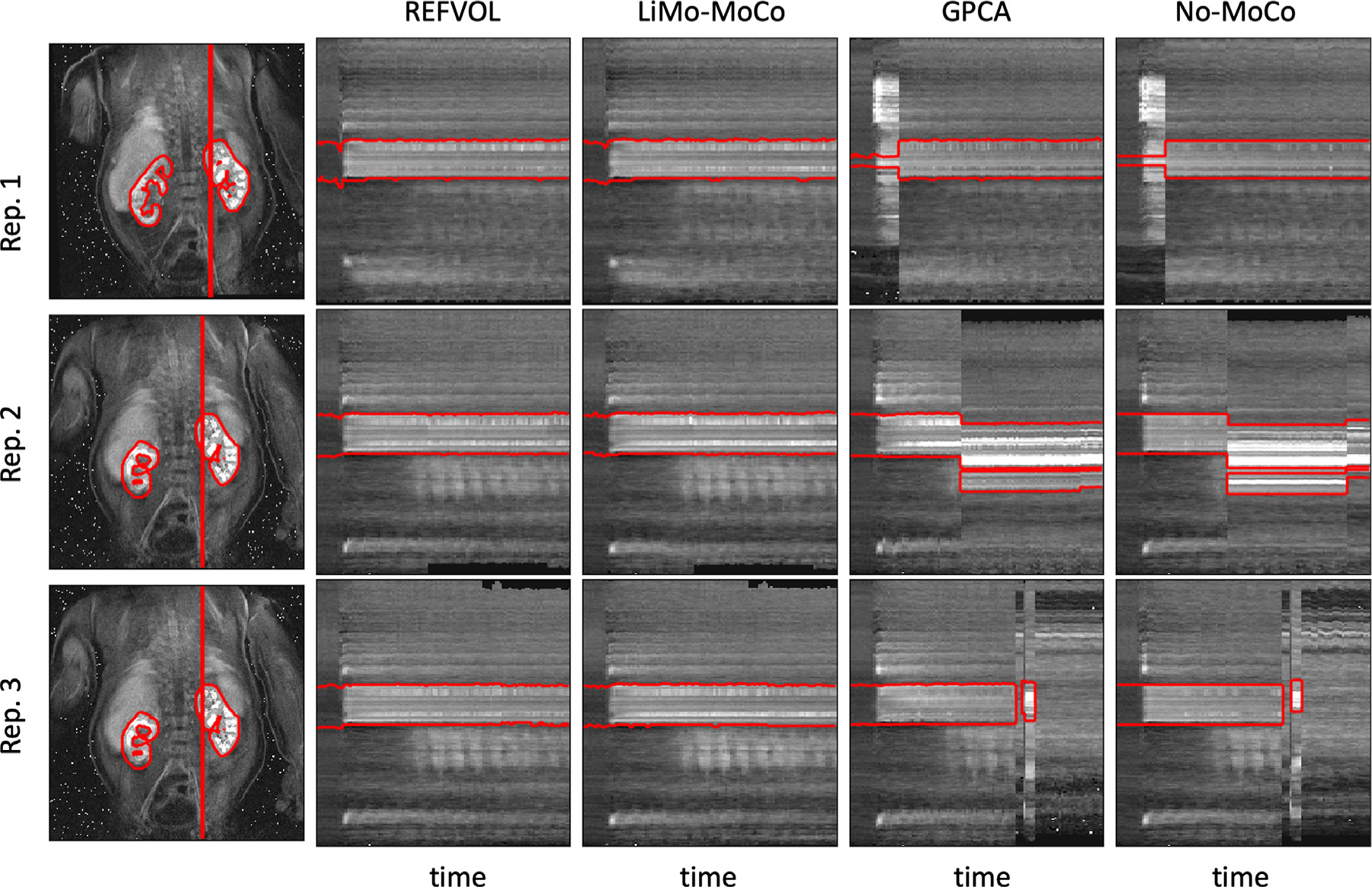
Line of voxels plotted over time for a sample repetition of the synthetic data experiment. Left, coronal reference image showing the line of voxels and the mask contour in red. Right, line of voxels over time for all registration methods (REFVOL, LiMo-MoCo, gPCA and No-MoCo). Overlaid, the section of the mask that corresponds to the voxels plotted. The No-MoCo panels present sharp discontinuities at the instances of motion that are corrected by the registration methods. Both REFVOL and LiMo-MoCo correctly align all the volumes, but REFVOL presents somewhat increased variability at the beginning of the sequence.

Table 1.

Summary results for the synthetic data experiments. The metrics shown in the table are the RMSE between ground truth and registered volumes (Volumes nRMSE), the DICE score between registered masks and the ground truth (Masks DICE), the percentage of times each kidney voxel was classified as such (Percent. kidney classification), the “Total Variation” metric of the concentration curves (TV), the estimation error of the parameters in the tracer kinetic model (F_P error and F_T error) and the residual of the model fit (Model fit nRMSE). LiMo-MoCo outperformed the other methods for all metrics except for the DICE score of the masks, for which REFVOL was more accurate.

Method	Volumes nRMSE	Masks DICE	Mask consistency (%)	TV	FP error [ml/100ml/min]	FT error[ml/100ml/min]	Model fit nRMSE
No-MoCo	2.267 ± 0.053	0.803 ± 0.295	54.8 ± 11.8	20.400 ± 2.920	79.7 ± 80.6	94.7 ± 1.338	0.283 ± 0.082
REFVOL	1.519 ± 0.102	0.958 ± 0.056	71.8 ± 2.3	14.180 ± 2.478	94.3 ± 122.0	72.5 ± 125.9	0.079 ± 0.009
gPCA	1.632 ± 0.049	0.523 ± 0.193	72.5 ± 15.0	19.704 ± 2.536	94.6 ± 114.6	109.3 ± 151.9	0.249 ± 0.053
LiMo-MoCo	1.514 ± 0.097	0.953 ± 0.051	74.1 ± 2.0	10.212 ± 1.499	75.6 ± 94.3	70.6 ± 123.2	0.065 ± 0.016

Fig. 3.

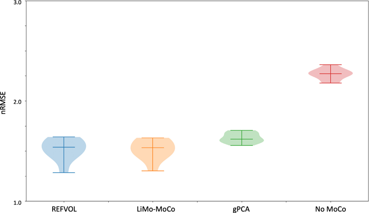
Box plot of the nRMSE between registered and ground truth volumes in the synthetic data experiments. The mean error due to alignment before registration is 2.67 in normalized units. Registration reduces the difference to 1.514 for LiMo-MoCo, 1.519 for REFVOL and 1.632 for gPCA. Both LiMo-MoCo and REFVOL attained the smallest nRMSE of the registered images.

Fig. 4 shows the consistency maps of three representative repetitions of the synthetic experiment. These show good agreement between the registered masks and the ground truth as well as high consistency over time. The discontinuities observed in Fig. 2, can be seen here as voxels with values greater than 0% but smaller than 100% outside of the ground truth mask.

Fig. 4.

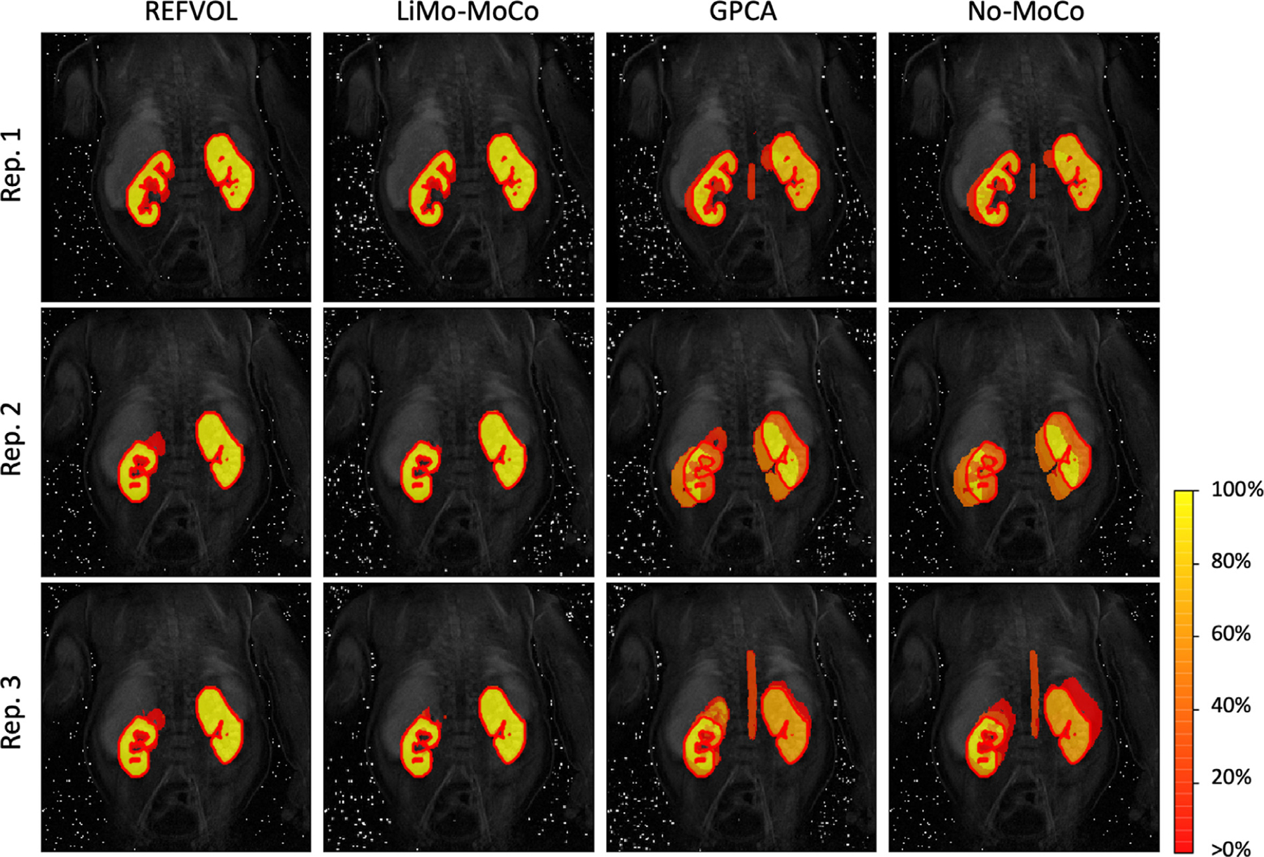
Consistency maps with the contours of the true kidney masks for three representative repetitions of the synthetic data experiment. The maps indicate the percentage of time that a voxel has been classified as kidney for each experiment. Voxels with values ∼ 100% indicate that these were consistently classified as kidney, while voxels with values between 0% and 100% shifted classification during the sequence. The masks registered with the different algorithms present good alignment with the ground truth masks. However, most algorithms present shifts in position of the mask in 10% of the time. LiMo-MoCo was the most consistent method in time while attaining similar accuracy values with the other competing methods (DICE coefficient 0.953).

Numerically, the misalignment with the ground truth resulted in a DICE value of 0.953 ± 0.051 for LiMo-MoCo, 0.958 ± 0.056 for REFVOL, 0.523 ± 0.193 for gPCA and 0.803 ± 0.295 No-Moco (Fig. 5). The DICE coefficient for LiMo-MoCo was higher than gPCA (p = 7.3 · 10⁻⁸) and No-MoCo (5.15 · 10⁻³), but not REFVOL (p = 1.9 · 10⁻⁴). The voxels within the region of interest were selected as kidney 74.1% of the time in LiMo-MoCo, 71.8% in REFVOL (p = 1.58 · 10⁻⁴), 47.3% in gPCA (p = 1.57 · 10⁻¹²) and 54.8% in No-MoCo ( p = 3.51 · 10⁻⁴). These results suggest that, both REFVOL and LiMo-MoCo achieved comparably accurate masks, but LiMo-Moco attained improved stability over time compared to REFVOL.

Fig. 5.

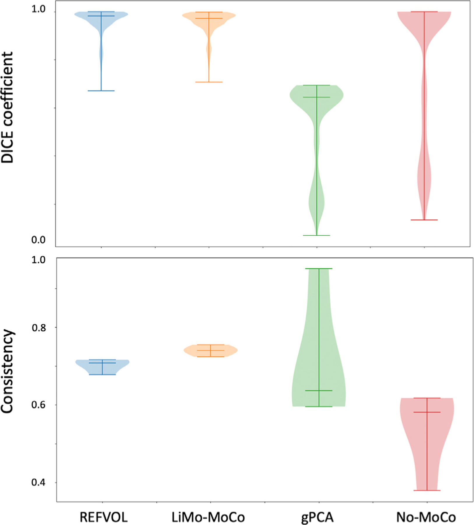
Top: Box plots with the DICE measure between the true mask and the masks aligned using the registration transforms. Bottom: Box plots of the average consistency of the registered masks. Both LiMo-MoCo and REFVOl attained the highest DICE coefficient (0.953 and 0.958), however, the masks registered with LiMo-MoCo were more self-consistent than the rest of the algorithms.

To measure the effect of registration variability on the concentration curves, we plot the TV metric on the concentration curves in Fig. 6. On average, the TV metric was smaller for LiMo-MoCo (10.212 ± 1.5) compared to REFVOL (14.180 ± 2.5, p = 6.3 · 10⁻⁵), gPCA (11.205 ± 1.3, p = 0.24) and No-Moco (20.4 ± 2.920, p = 7.4 · 10⁻⁷). Further suggesting that LiMo-MoCo was more consistent over time than the other methods.

Fig. 6.

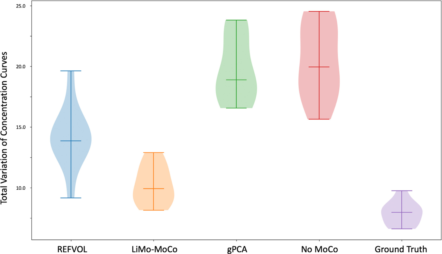
Total Variation metric applied to the concentration curves after registration of the synthetic data experiments. The metric computes the difference in absolute value between the concentration curves before and after applying Gaussian smoothing. LiMo-MoCo presented the smallest variability of all registration methods, indicating that it reduced the discontinuities created by motion.

Finally, we report on the tracer kinetic fitting results. The parameter maps for F_P and F_T are shown in Fig. 7 alongside with the corresponding nRMSE of the fitting procedure. For all cases, the parameter maps for both filtration rates show a clear distinction between the cortex and the medulla, similar to the maps generated with the ground truth. The residual maps presented higher differences across registration methods. LiMo-MoCo and REFVOL attained lower error in the cortex although the residual in the medulla was higher.

Fig. 7.

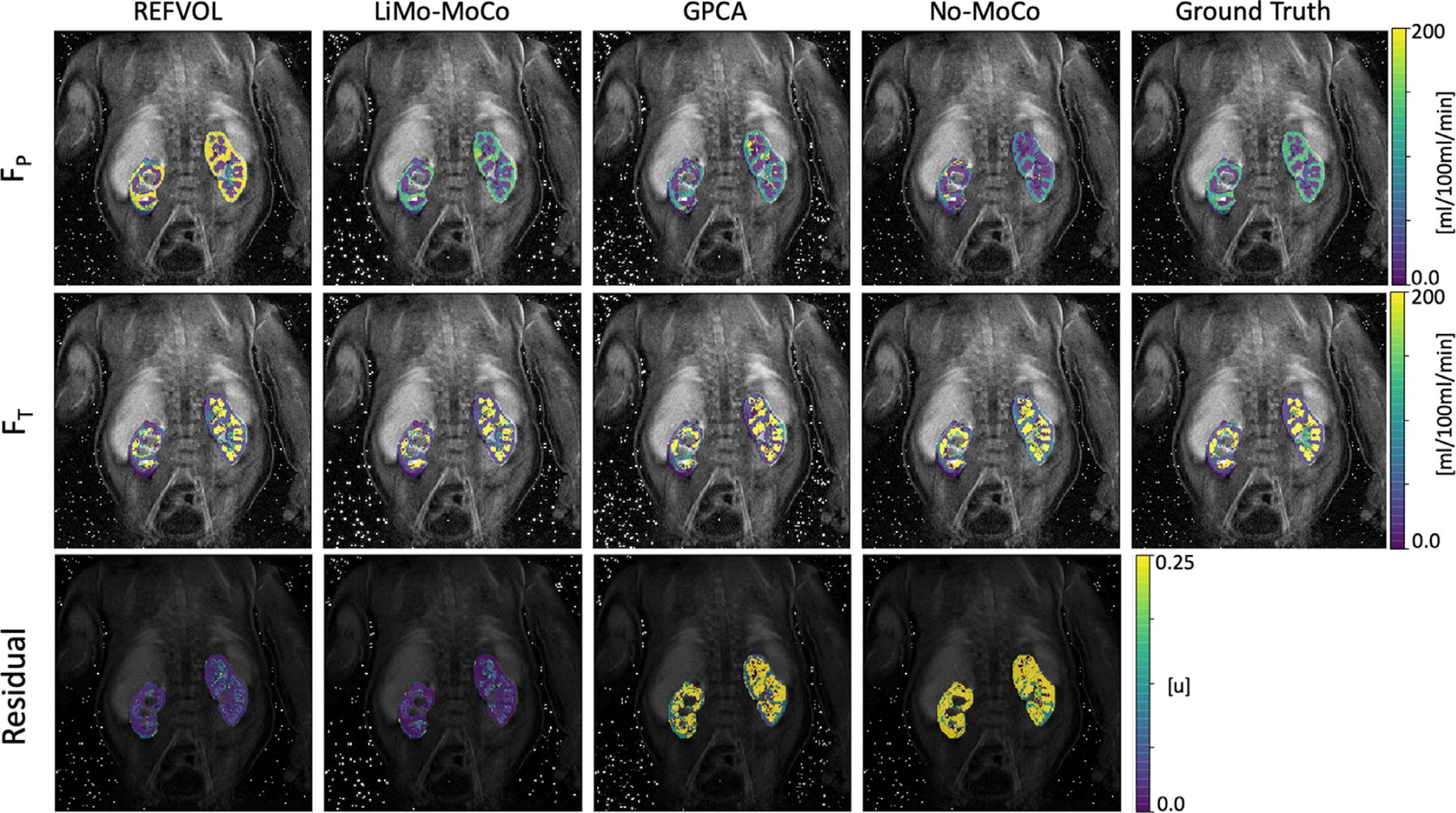
Parameter maps obtained after fitting the tracer kinetic model to the registered data and ground truth in one repetition of the synthetic experiment. The maps show the perfusion F_P, the tubular flow F_T and the nRMSE of the model fit (i.e. the goodness of fit). The parameter maps obtained with LiMo-MoCo present the highest similarity with the ground truth (average error in F_T = 66 ± 125 and F_P = 48 ± 62). Moreover, the residual error achieved with the proposed LiMo-MoCo was the smallest compared to other competing methods (0.94 ± 4.86).

The numerical results indicate that the proposed LiMo-MoCo method achived the lowest the average error in estimating the F_P parameter (75.6 ± 94.3 [ml/100ml/min]) compared to No-MoCo, REFVOL and gPCA techniques, which achieved an error of 79.7 ± 86.1, 94.3 ± 122.0 and 94.6 ± 114.6, respectively. Similarly, the proposed LiMo-MoCo method achieved the lowest average error in estimating the F_T parameter (70.6 ± 123.2) compared to No-MoCo, REFVOL and gPCA techniques, which achieved an error of 94.7 ± 133.8, 72.5 ± 125.9 and 109.3 ± 151.9, respectively. The differences were significant between LiMo-MoCo and gPCA (p = 0.0033), but not for LiMo-MoCo and REFVOL (p = 0.183) or No-MoCo (p = 0.0837).

On average, the nRMSE of the proposed LiMo-MoCo approach was smallest, with values of 0.065 ± 0.016 compared to 0.283 ± 0.082 for No-MoCo, 0.079 ± 0.009 for REFVOL and 0.249 ± 0.053 for gPCA. Here, the differences in nRMSE were statistically significant between LiMo-MoCo and gPCA, as well as between LiMo-Moco and No-MoCo (with p-values 1.54 · 10⁻⁶ and 1.76 · 10⁻⁵), but not for REFVOL (with p = 0.025).

4.2. Real data results

We first show the line plots from three sample subjects in Fig. 8. The plots correspond to a subject who presented small but continuous motion (A), a subject who showed larger and continuous motion at the start of the scan (B) and a subject who showed large sudden bulk motion at discrete instances of time (C). Broadly, all plots show the temporal evolution of each voxel undergoing the changes of intensity expected from the contrast agent intake with some discontinuities and distortions due to motion. However, there are some differences compared to the synthetic data experiments that must be addressed. Due to the nature of the MRI data acquisition, the reconstructed volumes present streaking artifacts and increased noise during motion events. In some cases, rapid bulk motion events result in signal dropout, which creates sudden outliers in time. These are particularly evident in the line plots of subject (C).

Fig. 8.

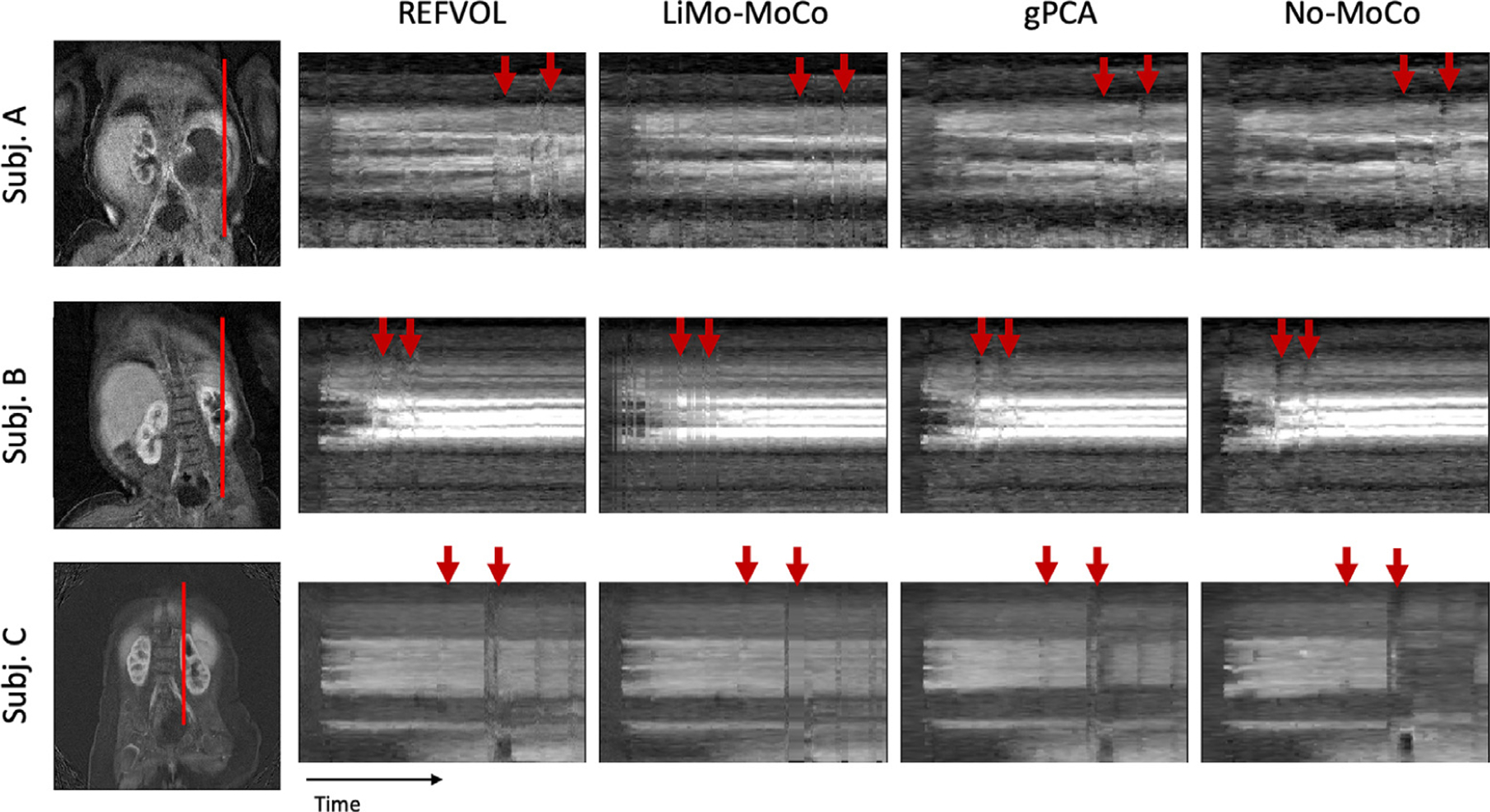
Line of voxels plotted over time for example subjects in the patient data experiments. Left, coronal reference image showing the line of voxels in red. Right, line of plots for all registration methods and the No-MoCo baseline. Before registration, the voxel intensities present small oscillations, sharp discontinuities and outliers (indicated with red arrows). All registration methods corrected the small oscillations and most discontinuities. The “Total Variation” metric for the three subjects was (0.456, 0.232 and 0.354) for LiMo-MoCo, (0.498, 0.284 and 0.420) for REFVOL, (0.469, 0.261 and0.407) for gPCA and (0.451, 0.311 and 0.419) for No-MoCo. LiMo-MoCo consistently aligned the volumes in time and corrected the volumes corrupted by motion with the LTI model.

All registration methods were capable of aligning the volumes and correcting the majority of discontinuities and distortions from the original No-MoCo cases. However, some small errors remained, particularly in areas with continued motion and increased noise. These are indicated in Fig. 2 with red arrows and appear as small discontinuities in the contrast lines. One particular alignment error that remained for gPCA were the sudden changes in position observed in subject (C). These, combined with the lower performance of gPCA in the synthetic data experiments, suggest that this method is insensitive to rapid bulk motion events and is better suited to correct for smooth motion such as respiration.

Fig. 9 illustrates the temporal behavior of the DCE signal in time before and after registration. Before motion correction, the volumes in the first part of the sequence (t₁ and t₂) were misaligned with the last section (t₄). Moreover, the volume acquired during motion (t₃) was corrupted and presented large signal dropout. Consequently, the corresponding intensity curves presented large discontinuities and signal dropout. The LTI model could capture the temporal behavior despite the motion artifacts and the proposed LiMo-MoCo method successfully aligned the volumes and could effectively interpolate those corrupted with signal dropout due to motion. The resulting curves after motion correction were smoother and had lower TV metric compared to those obtained with No-MoCo. The concentration curves obtained with the LiMo-MoCo results were smoother (0.244 ± 0.126) than those obtained with REFVOL (0.728 ± 1.831), gPCA (0.258 ± 0.170) and No-MoCo (0.295 ± 0.220). These differences were not statistically significant when averaged over all subjects (REFVOL p = 0.281, gPCA p = 0.389 and No-MoCo p = 0.091), but for subjects that presented motion (such as the ones shown in the Figures), the proposed technique significantly improved the performance.

Fig. 9.

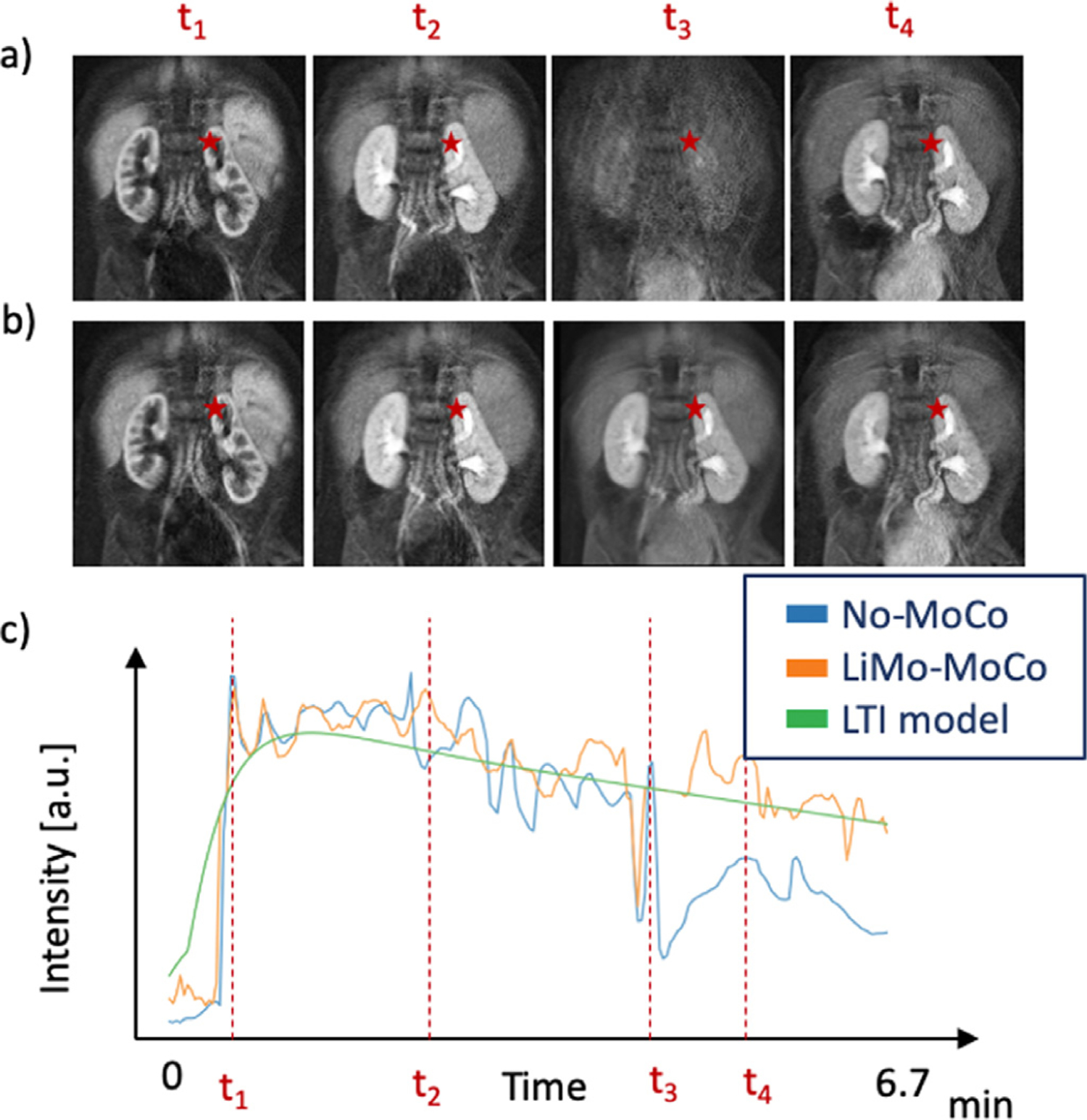
Illustration of the temporal behavior before and after registration of a subject. Panels (a) and (b) illustrate coronal images for No-MoCo and after applying LiMo-MoCo, respectively. Panel (c) shows the signal intensity of a single voxel for No-MoCo, LiMo-MoCo and the LTI model. The position of the voxel is indicated with the red star in the coronal images and the dashed lines in panel (c) indicate the times at which the volumes in panels (a) and (b) were acquired. Before registration, the subject changes position between frames t₂ and t₄. During the motion event, the images become corrupted and all the signal is lost. LiMo-MoCo correctly aligns the sequence of volumes and inpaints the corrupted volume with the LTI model. The Total Variation metric after registration was 0.35 compared to 0.42 in the No-MoCo case.

Fig. 10 shows the estimated parameter maps of each example subject. After registration the parameter maps were less noisy and the cortex and medulla structures could be differentiated. This was particularly clear for subject C, whose medulla was not visible in the No-Moco results, but appeared after motion correction. Moreover, the parameters estimated on the cortex matched those previously reported in the literature (e.g. F_T ∼ 40 – 100 ml/100ml/min and F_P ∼ 200 – 800ml/100ml/min). Similarly, the residual error of the tracer kinetic model fit was reduced after motion correction. This was particularly evident in the areas near edges of the tissue. For example, in the areas of transition between medulla and cortex (e.g. subject A), and at the boundaries of the kidney (e.g. subject B). In the case of subject C, the original error was high throughout the kidney (∼ 0.01) and motion-correction showed minor improvement.

Fig. 10.

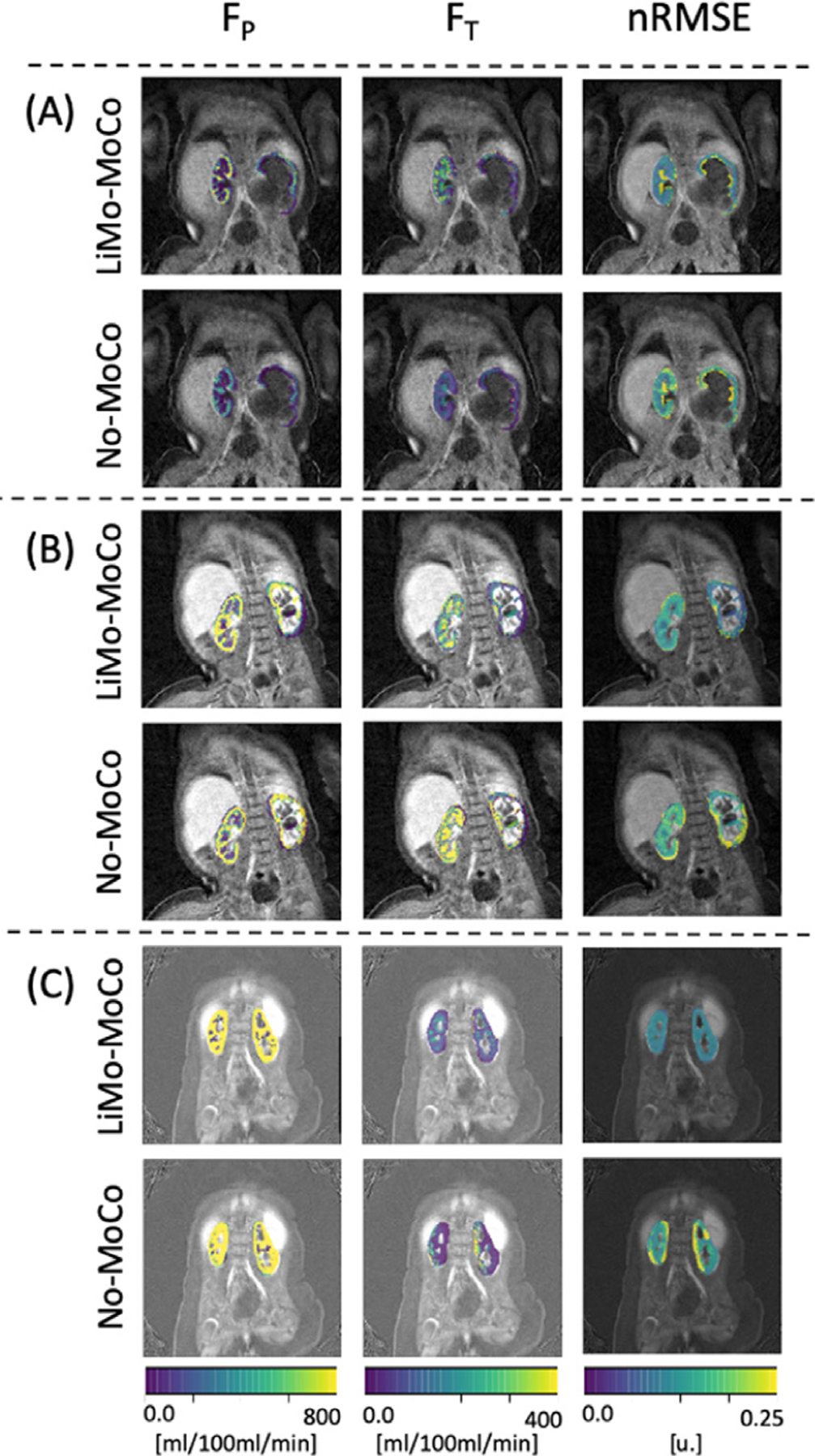
Results of the tracer kinetic fit. Comparison between LiMo-MoCo and No-Moco of three representative subjects of the patient data experiments. Left and middle columns correspond to the filtration parameters (F_P and F_T) and right column corresponds to the nRMSE of the model fit. The nRMSE for the three subjects was (0.172, 0.102 and 0.105) for LiMo-MoCo, (0.236, 0.010 and 0.107) for REFVOL, (0.175, 0.123 and 0.128) for gPCA, (0.241, 0.147 and 0.151) for No-MoCo.After registration with LiMo-MoCo, the residual is reduced and the parameter maps allow to distinguish the cortex from the medulla of each subject.

All registration methods improved the goodness of fit of the tracer kinetic model but LiMo-MoCo performed best. The median nRMSE was 0.109 ± 0.184 for LiMo-MoCo, 0.117 ± 0.227 for REFVOL, 0.111 ± 0.184 for gPCA and 0.143 ± 0.185 for No-MoCo. Only the difference between LiMo-MoCo and No-MoCo were statistically significant (0.35 for REFVOL, 0.94 for gPCA and 0.038 for No-MoCo).

Computationally, REFVOL was the fastest algorithm with an average compute time of 22.5 ± 8.7 min, LiMo-MoCo was second with a compute time of 132.9 ± 26.8 min and gPCA last with 1.1 ± 0.23 days. The LiMo-MoCo algorithm was implemented in python and the registration time accounted for ∼ 22 min (same as the REFVOL results) while the LTI model fit added 75.9 ± 17.9 per iteration.

5. Conclusions and discussion

We presented an LTI model based motion correction (LiMo-MoCo) approach for DCE-MR images of the kidneys. Our approach characterizes the DCE-MRI data over time as the response of an LTI system to the injection of the contrast agent into the blood stream. Our results suggest that this method provides a more consistent registration of volumes over the time and it helps improve the accuracy of the tracer kinetic model fitting. The results indicate that all registration methods improved alignment although each method had different weaknesses. REFVOL provided the most accurate registration of the masks, but at the cost of increased variability over time, which reduced the accuracy of the tracer kinetic model fitting. GPCA performed well to register patient DCE-MRI data. Its metric, which measures the variance of the volumes in time, is well suited to characterize small and repeated motion such as respiration. However, it might not be sensitive to sudden bulk motion events –e.g. rapid changes in position of the subject. LiMo-MoCo performed consistently well for all types of motion and presented reduced variability in time compared to REFVOL.

LiMo-Moco is a model-based approach to registration and is similar to other model based approaches developed for DCE-MRI Buonaccorsi et al. (2007). However, the tracer kinetic models used in previous work are sensitive to the underlying tissue type and require pre-defining a region of interest to which they can be reliably fitted. Instead, the LTI model used in LiMo-MoCo allows to characterize each voxel in the field of view from different tissue types, and can perform well even in the presence of streaking artifacts and low signal-to-noise ratio, which reduce the quality of images and complicates the registration. Note that the algorithm used to fit the proposed LTI model based registration is essential to be robust to motion and streaking artifacts. Recent work proposed using TK models instead of an LTI model to perform joint parameter estimation and registration Dikaios (2020) using a data driven optimization scheme. Because a single TK model does not fit to all tissues types, they used a model selection step to determine which model is best suited for each different tissue type. It would be interesting to incorporate the proposed optimization scheme into our proposed motion compensation framework in future work.

In this work, we used non-rigid registration with the aim of correcting for non-rigid motion such as pulsatile motion and non-rigid deformations of the other organs and especially aorta, which is important to accurately measure to generate an accurate AIF. However, our approach can be readily modified to register each kidney with rigid alignment.

Beyond registration, the presented LTI model has been used to recover and reconstruct corrupted volumes acquired during the motion events. It also has several other applications. The template volumes of the entire field of view generated with the LTI model can be used as a denoising technique Gal et al. (2010). Here, the algorithm would solve an optimization problem similar to Total-Variation denoising, but with a regularization term enforcing similarity to the template volumes. Similarly, the LTI model could be used to regularize sparse image reconstruction methods from sparse k-space data acquired with radial or cartesian sampling schemes Ippoliti et al. (2019); Hausmann et al. (2019). For both applications, the LTI model would serve as a parsimonious representation of the temporal dynamics of the data. Moreover, since the optimization of the LTI model parameters is robust to artifacts it could be applied even in applications where the noise is not Gaussian.

The main limitation of this work, as for all studies evaluating motion compensation techniques, is the lack of an established validation standard for registration. To overcome this limitation, we assessed the results with a variety of metrics including those assessing properties of the geometry (DICE score and consistency), as well as the TK model fit (TV and nRMSE), whose improvement is the ultimate goal of this work. However, without a consensus on what are the best metrics for validation, any combination of metrics will be limited Zöllner et al. (2019). The lack of ground truth for the real data is also a limitation of this study. We tried addressing this issue by using a synthetic model, for which we have ground truth. Future work with synthetic models should incorporate more realistic characterizations of the various kinds of motion and apply them to data before image reconstruction to simulate both realistic motion and undersampling artifacts in the simulated images.

References

- Adluru G, DiBella EV, Schabel MC, 2006. Model-based registration for dynamic cardiac perfusion MRI. J. Magn. Reson. Imaging 24 (5), 1062–1070. 10.1002/jmri.20756. [DOI] [PubMed] [Google Scholar]
- Block KT, Chandarana H, Milla S, Bruno M, Mulholland T, Fatterpekar G, Hagiwara M, Grimm R, Geppert C, Kiefer B, Sodickson DK, 2014. Towards routine clinical use of radial stack-of-Stars 3D gradient-echo sequences for reducing motion sensitivity. Journal of the Korean Society of Magnetic Resonance in Medicine 18 (2), 87 10.13104/jksmrm.2014.18.2.87. [DOI] [Google Scholar]
- Buonaccorsi GA, O’Connor JP, Caunce A, Roberts C, Cheung S, Watson Y, Davies K, Hope L, Jackson A, Jayson GC, Parker GJ, 2007. Tracer kinetic model-driven registration for dynamic contrast-enhanced MRI time-series data. Magn Reson Med 58 (5), 1010–1019. 10.1002/mrm.21405. [DOI] [PubMed] [Google Scholar]
- Buonaccorsi GA, Roberts C, Cheung S, Watson Y, Davies K, Jackson A, Jayson GC, Parker GJ, 2005. Tracer kinetic model-driven registration for dynamic contrast enhanced MRI time series. In: Lecture Notes in Computer Science (including subseries Lecture Notes in Artificial Intelligence and Lecture Notes in Bioinformatics), 3749 LNCS, pp. 91–98. 10.1007/11566465_12. [DOI] [Google Scholar]
- Buonaccorsi GA, Roberts C, Cheung S, Watson Y, O’Connor JP, Davies K, Jackson A, Jayson GC, Parker GJ, 2006. Comparison of the performance of tracer kinetic model-driven registration for dynamic contrast enhanced MRI using different models of contrast enhancement. Acad Radiol 13 (9), 1112–1123. 10.1016/j.acra.2006.05.016. [DOI] [PubMed] [Google Scholar]
- Caldeira L, Sanches J, 2008. Liver tumor assessment with DCE-MRI. In: 2008 5th IEEE International Symposium on Biomedical Imaging: From Nano to Macro, Proceedings, ISBI, pp. 804–807. 10.1016/j.acra.2006.05.016. [DOI] [Google Scholar]
- Chandarana H, Block KT, Winfeld MJ, Lala SV, Mazori D, Giuffrida E, Babb JS, Milla SS, 2014. Free-breathing contrast-enhanced T1-weighted gradient-echo imaging with radial k-space sampling for paediatric abdominopelvic MRI. Eur Radiol 24 (2), 320–326. 10.1007/s00330-013-3026-4. [DOI] [PubMed] [Google Scholar]
- Chandarana H, Feng L, Ream J, Wang A, Babb JS, Block KT, Sodickson DK, Otazo R, 2015. Respiratory motion-Resolved compressed sensing reconstruction of free-Breathing radial acquisition for dynamic liver magnetic resonance imaging. Invest Radiol 50 (11), 749–756. 10.1097/RLI.0000000000000179. [DOI] [PMC free article] [PubMed] [Google Scholar]
- Chevalier RL, 1995. Effects of ureteral obstruction on renal growth. Semin. Nephrol. 15 (4), 353–360. [PubMed] [Google Scholar]
- Chevalier RL, Thornhill BA, Forbes MS, Kiley SC, 2010. Mechanisms of renal injury and progression of renal disease in congenital obstructive nephropathy. Pediatric Nephrology 25 (4), 687–697. 10.1007/s00467-009-1316-5. [DOI] [PubMed] [Google Scholar]
- Coll-Font J, Afacan O, Chow J, Kurugol S, 2019. Linear Time Invariant Model Based Motion Correction (LiMo-MoCo) of Dynamic Radial Contrast Enhanced MRI In: Lecture Notes in Computer Science (including subseries Lecture Notes in Artificial Intelligence and Lecture Notes in Bioinformatics). Springer, pp. 430–437. 10.1007/978-3-030-32245-8_48. [DOI] [PMC free article] [PubMed] [Google Scholar]
- Coll-Font J, Afacan O, Chow JS, Lee RS, Stemmer A, Warfield SK, Kurugol S, 2019. Bulk motion-compensated DCE-MRI for functional imaging of kidneys in newborns. J. Magn. Reson. Imaging 10.1002/jmri.27021. [DOI] [PMC free article] [PubMed]
- Coll-Font J, Afacan O, Stemmer A, Lee RS, Chow JS, Warfield SK, Kurugol S, 2019. Self-navigated bulk motion detection for feed and wrap renal dynamic radial VIBE DCE-MRI. In: International Society for Magnetic Resonance in Medicine (ISMRM).
- Dikaios N, 2020. Stochastic Gradient Langevin dynamics for joint parameterization of tracer kinetic models, input functions, and T1 relaxation-times from undersampled k-space DCE-MRI. Med Image Anal 62, 101690 10.1016/j.media.2020.101690. [DOI] [PubMed] [Google Scholar]
- Fei B, Flask C, Hesheng W, Pi A, Wilson DL, Shillingford J, Murcia N, Weimbs T, Duerk JL, 2005. Image segmentation, registration and visualization of serial MR images for therapeutic assessment of polycystic kidney disease in transgenic mice. In: Annual International Conference of the IEEE Engineering in Medicine and Biology - Proceedings, 7 VOLS, pp. 467–469. 10.1109/iembs.2005.1616448. [DOI] [PubMed] [Google Scholar]
- Feng L, Grimm R, Block KTT, Chandarana H, Kim S, Xu J, Axel L, Sodickson DK, Otazo R, 2014. Golden-angle radial sparse parallel MRI: combination of compressed sensing, parallel imaging, and golden-angle radial sampling for fast and flexible dynamic volumetric MRI. Magn Reson Med 72 (3), 707–717. 10.1002/mrm.24980. [DOI] [PMC free article] [PubMed] [Google Scholar]
- Gal Y, Mehnert AJ, Bradley AP, McMahon K, Kennedy D, Crozier S, 2010. Denoising of dynamic contrast-enhanced MR images using dynamic nonlocal means. IEEE Trans Med Imaging 29 (2), 302–310. 10.1109/TMI.2009.2026575. [DOI] [PubMed] [Google Scholar]
- Grattan-Smith JD, Little SB, Jones RA, 2008. MR urography evaluation of obstructive uropathy. Pediatr Radiol 38 (1 SUPPL.), 49–69. 10.1007/s00247-007-0667-y. [DOI] [PubMed] [Google Scholar]
- Haghighi M, Warfield SK, Kurugol S, 2018. Automatic renal segmentation in DCE-MRI using convolutional neural networks. In: 2018 IEEE 15th International Symposium on Biomedical Imaging (ISBI 2018) IEEE, pp. 1534–1537. 10.1109/ISBI.2018.8363865. [DOI] [PMC free article] [PubMed] [Google Scholar]
- Hamy V, Dikaios N, Punwani S, Melbourne A, Latifoltojar A, Makanyanga J, Chouhan M, Helbren E, Menys A, Taylor S, Atkinson D, 2014. Respiratory motion correction in dynamic MRI using robust data decomposition registration - Application to DCE-MRI. Med Image Anal 18 (2), 301–313. 10.1016/j.media.2013.10.016. [DOI] [PubMed] [Google Scholar]
- Hausmann D, Niemann T, Kreul D, Nocito A, Klarhöfer M, Nickel DM, Kiefer B, Attenberger UI, Zöllner FG, Kubik-Huch RA, 2019. Free-Breathing dynamic contrast-enhanced imaging of the upper abdomen using a cartesian compressed-Sensing sequence with hard-Gated and motion-State-Resolved reconstruction. Invest Radiol 54 (11), 728–736. 10.1097/RLI.0000000000000607. [DOI] [PubMed] [Google Scholar]
- Hodneland E, Hanson EA, Lundervold A, Modersitzki J, Eikefjord E, Munthe-Kaas AZ, 2014. Segmentation-driven image registration-application to 4D DCE-MRI recordings of the moving kidneys. IEEE Trans. Image Process 23 (5), 2392–2404. 10.1109/TIP.2014.2315155. [DOI] [PubMed] [Google Scholar]
- Hodneland E, Lundervold A, Rørvik J, Munthe-Kaas AZ, 2014. Normalized gradient fields for nonlinear motion correction of DCE-MRI time series. Computerized Medical Imaging and Graphics 38 (3), 202–210. 10.1016/j.compmedimag.2013.12.007. [DOI] [PubMed] [Google Scholar]
- Huizinga W, Poot D, Guyader J-M, Klaassen R, Coolen B, van Kranenburg M, van Geuns R, Uitterdijk A, Polfliet M, Vandemeulebroucke J, Leemans A, Niessen W, Klein S, 2016. PCA-Based groupwise image registration for quantitative MRI. Med Image Anal 29, 65–78. 10.1016/j.media.2015.12.004. [DOI] [PubMed] [Google Scholar]
- Ingrisch M, Sourbron S, 2013. Tracer-kinetic modeling of dynamic contrast-enhanced MRI and CT: a primer. J Pharmacokinet Pharmacodyn 40 (3), 281–300. 10.1007/s10928-013-9315-3. [DOI] [PubMed] [Google Scholar]
- Ippoliti M, Lukas M, Brenner W, Makowski MR, Kolbitsch C, Kolbitsch C, Schaeffter T, Makowski MR, Kolbitsch C, 2019. 3D Nonrigid motion correction for quantitative assessment of hepatic lesions in DCE-MRI. Magn Reson Med 82 (5), 1753–1766. 10.1002/mrm.27867. [DOI] [PMC free article] [PubMed] [Google Scholar]
- Jaggi M, 2013. Revisiting Frank-Wolfe: projection-free sparse convex optimization. Proceedings of the 30th International Conference on Machine Learning 28, 427–435. [Google Scholar]
- Johansson A, Balter J, Feng M, Cao Y, 2016. An overdetermined system of transform equations in support of robust DCE-MRI registration with outlier rejection. Tomography (Ann Arbor, Mich.) 2 (3), 188–196. 10.18383/j.tom.2016.00145. [DOI] [PMC free article] [PubMed] [Google Scholar]
- Khalifa F, Soliman A, El-Baz A, Abou El-Ghar M, El-Diasty T, Gimel’Farb G, Ouseph R, Dwyer AC, 2014. Models and methods for analyzing DCE-MRI: areview. Med Phys 41 (12). 10.1118/1.4898202. [DOI] [PubMed] [Google Scholar]
- Klein S.e., 2010. Elastix: A Toolbox for intensity-Based medical image registration. IEEE Trans Med Imaging 29 (1), 196–205. 10.1109/TMI.2009.2035616. [DOI] [PubMed] [Google Scholar]
- Kurugol S, Afacan O, Lee RS, Seager CM, Ferguson MA, Stein DR, Nichols RC, Dugan M, Stemmer A, Warfield SK, Chow JS, 2020. Prospective pediatric study comparing glomerular filtration rate estimates based on motion-robust dynamic contrast-enhanced magnetic resonance imaging and serum creatinine (egfr) to 99mtc DTPA. Pediatr Radiol 10.1007/s00247-020-04617-0. [DOI] [PMC free article] [PubMed]
- Kurugol S, Afacan O, Seager C, Lee RS, Chow JS, Warfield SK, 2018. Compensating for Bulk Motion in Feed and Wrap Renal Dynamic Radial VIBE DCE-MRI using Bulk Motion Removal and Non-Rigid Registration. In: International Society for Magnetic Resonance in Medicine (ISMRM), pp. 72–74.
- Kurugol S, Ferguson MA, Seethamraju RT, 2017. Reliable estimation of kidney filtration rate with DCE-MRI using motion-robust high spatiotemporal resolution Radial VIBE Speech Imaging View project Real-Time Deformable (non-rigid) Registration for 3D Brain MRI View project. In: International Society for Magnetic Resonance in Medicine (ISMRM).
- Kurugol S, Freiman M, Afacan O, Domachevsky L, Perez-Rossello JM, Callahan MJ, Warfield SK, 2017. Motion-robust parameter estimation in abdominal diffusion-weighted MRI by simultaneous image registration and model estimation. Med Image Anal 39, 124–132. 10.1016/J.MEDIA.2017.04.006. [DOI] [PMC free article] [PubMed] [Google Scholar]
- Kurugol S, Seager CM, Thaker H, Coll-Font J, Afacan O, Nichols RC, Warfield SK, Lee RS, Chow JS, 2019. Feed and wrap magnetic resonance urography provides anatomic and functional imaging in infants without anesthesia. J Pediatr Urol 10.1016/j.jpurol.2019.11.002. [DOI] [PubMed]
- Melbourne A, Atkinson D, White MJ, Collins D, Leach M, Hawkes D, 2007. Registration of dynamic contrast-enhanced MRI using a progressive principal component registration (PPCR). Phys Med Biol 52 (17), 5147–5156. 10.1088/0031-9155/52/17/003. [DOI] [PubMed] [Google Scholar]
- Melbourne A, Hipwell J, Modat M, Mertzanidou T, Huisman H, Ourselin S, Hawkes DJ, 2011. The effect of motion correction on pharmacokinetic parameter estimation in dynamic-contrast-enhanced MRI. Phys Med Biol 56 (24), 7693–7708. 10.1088/0031-9155/56/24/001. [DOI] [PubMed] [Google Scholar]
- Merrem AD, Zöllner FG, Reich M, Lundervold A, Rorvik J, Schad LR, 2013. A variational approach to image registration in dynamic contrast-enhanced MRI of the human kidney. Magn Reson Imaging 31 (5), 771–777. 10.1016/j.mri.2012.10.011. [DOI] [PubMed] [Google Scholar]
- Michaely HJ, Sourbron SP, Buettner C, Lodemann KP, Reiser MF, Schoenberg SO, 2008. Temporal constraints in renal perfusion imaging with a 2-compartment model. Invest Radiol 43 (2), 120–128. 10.1097/RLI.0b013e3181583b0c. [DOI] [PubMed] [Google Scholar]
- Positano V, Bernardeschi I, Zampa V, Marinelli M, Landini L, Santarelli MF, 2013. Automatic 2D registration of renal perfusion image sequences by mutual information and adaptive prediction. Magn. Reson. Mater. Phys., Biol. Med 26 (3), 325–335. 10.1007/s10334-012-0337-4. [DOI] [PubMed] [Google Scholar]
- Sourbron S.P.e., 2008. MRI-Measurement of perfusion and glomerular filtration in the human kidney with a separable compartment model. Invest Radiol 43 (1), 40–48. 10.1097/RLI.0b013e31815597c5. [DOI] [PubMed] [Google Scholar]
- Wright KL, Chen Y, Saybasili H, Griswold MA, Seiberlich N, Gulani V, 2014. Quantitative high-resolution renal perfusion imaging using 3-dimensional through-time radial generalized autocalibrating partially parallel acquisition. Invest Radiol 49 (10), 666–674. 10.1097/RLI.0000000000000070. [DOI] [PMC free article] [PubMed] [Google Scholar]
- Yilmaz B, Bekiroglu K, Lagoa C, Sznaier M, 2018. A randomized algorithm for parsimonious model identification. IEEE Trans Automat Contr 63 (2), 532–539. 10.1109/TAC.2017.2723959. [DOI] [Google Scholar]
- Zöllner FG, Šerifović-Trbalić A, Kabelitz G, Kociński M, Materka A, Rogelj P, 2019. Image registration in dynamic renal MRI–current status and prospects. Magn. Reson. Mater. Phys., Biol. Med 33 (1), 33–48. 10.1007/s10334-019-00782-y. [DOI] [PMC free article] [PubMed] [Google Scholar]