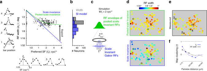
Fig. 3. Receptive field width as a function of preferred SF (fo).
a The scatter plot compares fo to RF width from three ROIs, each indicated by a different symbol. See Table 2 for joint statistics. The five data points at the extreme left of the x-axis were “low pass” (see “Methods”). To the left of the y-axis are position tuning curves (black dots) and Gaussian fits (gray) of four example neurons in one ROI outlined and enumerated in e. Below the x-axis are the SF tuning curves and fits of the same four cells. b Distribution of measured RF width and the scale invariance prediction of RF width based on fo. c Illustration of the pooling model in the spatial domain, at fo = 2 cyc/°. At bottom are the 1D Gabor functions from the model of scale invariance. They are shifted and weighted according to the Gaussian in the pooling model (σh(x) = 0.24°). The superposition of the Gabors’ energy (i.e. their envelopes) yields the wider green Gaussian on top, which is the output of the pooling model. d Bottom and top panels are the predicted map of RF width by plugging fo into the scale invariance model and pooled scale invariance model, respectively. The yield in these map are based on tuning fits to the random grating stimulus (see “Methods”). e Map of the measured RF width. The yield in d is different from e because they are based on tuning fits from two separate stimulus blocks, the random gratings and random bars (Fig. 2c, j), respectively. Like the map in e, the scatter plot in a showed the intersection of the yield between the two different stimulus blocks. f Pearson correlation coefficient between neuron pairs, within 75 μm cortical distance bins, using all three ROIs in the study. The symbol at each distance bin indicates the correlation coefficient’s significance: Closed dot is p > 0.01, asterisk is p < 0.01, asterisk and open circle is p < 0.001.

