Structural identifiability and observability of compartmental models of the COVID-19 pandemic

Abstract

The recent coronavirus disease (COVID-19) outbreak has dramatically increased the public awareness and appreciation of the utility of dynamic models. At the same time, the dissemination of contradictory model predictions has highlighted their limitations. If some parameters and/or state variables of a model cannot be determined from output measurements, its ability to yield correct insights – as well as the possibility of controlling the system – may be compromised. Epidemic dynamics are commonly analysed using compartmental models, and many variations of such models have been used for analysing and predicting the evolution of the COVID-19 pandemic. In this paper we survey the different models proposed in the literature, assembling a list of 36 model structures and assessing their ability to provide reliable information. We address the problem using the control theoretic concepts of structural identifiability and observability. Since some parameters can vary during the course of an epidemic, we consider both the constant and time-varying parameter assumptions. We analyse the structural identifiability and observability of all of the models, considering all plausible choices of outputs and time-varying parameters, which leads us to analyse 255 different model versions. We classify the models according to their structural identifiability and observability under the different assumptions and discuss the implications of the results. We also illustrate with an example several alternative ways of remedying the lack of observability of a model. Our analyses provide guidelines for choosing the most informative model for each purpose, taking into account the available knowledge and measurements.

1. Introduction

The current coronavirus disease (COVID-19) pandemic, caused by the SARS-CoV-2 virus, continues to wreak unparallelled havoc across the world. Public health authorities can use mathematical models to answer critical questions related with the dynamics of an epidemic (severity and time course of infected people), its impact on the healthcare system, and the design and effectiveness of different interventions (Adam, 2020, Currie et al., 2020, Li, 2018, Lofgren et al., 2014). Mathematical modelling of infectious diseases has a long history (Brauer et al., 2008, Martcheva, 2015). Modelling efforts are particularly important in the context of COVID-19 because its dynamics can be particularly complex and counter-intuitive due to the uncertainty in the transmission mechanisms, possible seasonal variation in both susceptibility and transmission, and their variation within subpopulations (Cobey, 2020). The media has given extensive coverage to analyses and forecasts using COVID-19 models, with increased attention to cases of conflicting conclusions, giving the impression that epidemiological models are unreliable or flawed. However, a closer look reveals that these modelling studies were following different approaches, handling uncertainty differently, and ultimately addressing different questions on different time-scales (Holmdahl & Buckee, 2020).

Broadly speaking, data-driven models (using statistical regression or machine learning) can be used for short-term forecasts (one or a few weeks). Mechanistic models based on assumptions about transmission and immunity try to mimic how the virus spreads, and can be used to formalize current knowledge and explore long-term outcomes of the pandemic and the effectiveness of different interventions. However, the accuracy of mechanistic models is constrained by the uncertainties in our knowledge, which creates uncertainties in model parameters and even in the model structure (Holmdahl & Buckee, 2020). Further, the uncertainty in the COVID-19 data and the exponential spread of the virus amplify the uncertainty in the predictions. Predictability studies (Scarpino & Petri, 2019) seek the characterization of the fundamental limits to outbreak prediction and their impact on decision-making. Despite the vast literature on mathematical epidemiology in general, and modelling of COVID-19 in particular, comparatively few authors have considered the predictability of infectious disease outbreaks (Castro et al., 2020, Scarpino and Petri, 2019). Uncertainty quantification (Arriola & Hyman, 2009) is an interconnected concept that is also key for the reliability of a model, and that has received similarly scant attention (Faranda et al., 2020, Raimúndez et al., 2020).

In addition to predictability and uncertainty quantification approaches, identifiability is a related property whose absence can severely limit the usefulness of a mechanistic model (Chowell, 2017). A model is identifiable if we can determine the values of its parameters from knowledge of its inputs and outputs. Likewise, the related control theoretic property of observability describes if we can infer the model states from knowledge of its inputs and outputs. If a model is non-identifiable (or non-observable) different sets of parameters (or states) can produce the same predictions or fit to data. The implications can be enormous: in the context of the COVID-19 outbreak in Wuhan, non-identifiability in model calibrations was identified as the main reason for wide variations in model predictions (Roda, Varughese, Han, & Li, 2020).

Reliable models can be used in combination with optimization and optimal control methods to find the best intervention strategies, such as lock-downs with minimum economic impact (Acemoglu et al., 2020, Alvarez et al., 2020). Further, they can be used to explore the feasibility of model-based real-time control of the pandemic (Casella, 2020, Köhler et al., 2020). However, using calibrated models with non-identifiability or non-observability issues can result in bad or even dangerous intervention and control strategies.

It is common to distinguish between structural and practical identifiability. Structural non-identifiability may be due to the model and measurement (input–output) structure. Practical non-identifiability is due to lack of information in the considered data-sets. Non-identifiability results in incorrect parameter estimates and bad uncertainty quantification (Chowell, 2017, Kao and Eisenberg, 2018), i.e. a misleading calibrated model which should not be used to analyse epidemiological data, test hypothesis, or design interventions. The structural identifiability of several epidemic mechanistic models has been studied e.g. in Brouwer et al., 2019, Chapman and Evans, 2009, Eisenberg et al., 2013, Evans et al., 2002, Evans et al., 2005, Prague et al., 2020. Other recent studies have mostly focused on practical identifiability, such as Alahmadi et al., 2020, Chowell, 2017, Kao and Eisenberg, 2018, Roosa and Chowell, 2019, Tuncer and Le, 2018.

Since checking structural identifiability can be hard, one might think that directly checking practical identifiability could be a better alternative. However, it has been shown Janzén et al. (2016) that this practice entails at least two dangers: (i) checking practical identifiability can exhibit numerical issues that lead to wrong results, and (ii) if structural identifiability is unknown, the source of uncertainty in the parameter estimates can be either the data or the model structure, so it will not be clear how to improve the situation. In contrast, if we can verify structural identifiability, we can then focus on the data uncertainty to resolve possible practical identifiability issues. In other words, practical identifiability analysis cannot be used to deduce structural identifiability, and ignoring the latter can lead to modelling artefacts.

In this paper we assess the structural identifiability and observability of a large set of COVID-19 mechanistic models described by deterministic ordinary differential equations, derived by different authors using the compartmental modelling framework (Brauer, 2008). Compartmental models are widely used in epidemiology because they are tractable and powerful despite their simplicity. We collect 36 different compartmental models, of which we consider several variations, making up a total of 255 different model versions. Our aim is to characterize their ability to provide insights about their unknown parameters – i.e. their structural identifiability – and unmeasured states – i.e. their observability. To this end we adopt a differential geometry approach that considers structural identifiability as a particular case of nonlinear observability, allowing to analyse both properties jointly. We define the relevant concepts and describe the methods used in Section 2. Then we provide an overview of the different types of compartmental models found in the literature in Section 3. We analyse their structural identifiability and observability and discuss the results in Section 4, where we also show different ways of remedying lack of observability using an illustrative model. Finally, we conclude our study with some key remarks in Section 5.

2. Methods

2.1. Notation, models, and properties

We consider models defined by systems of ordinary differential equations with the following notation:

$$\mathcal{M}=\left\{\begin{array}{cc}\dot{x}\left(t\right)=f\left(x\left(t\right),\theta ,u\left(t\right),w\left(t\right)\right)\hfill & \mathrm{(a)}\hfill \\ y\left(t\right)=h\left(x\left(t\right),\theta ,u\left(t\right),w\left(t\right)\right)\hfill & \mathrm{(b)}\hfill \end{array}\right)$$ (1)

where $f$ and $h$ are analytical (generally nonlinear) functions of the states $x\left(t\right)\in {\mathbb{R}}^{n_x}$, known inputs $u\left(t\right)\in {\mathbb{R}}^{n_u}$, unknown constant parameters $\theta \in {\mathbb{R}}^{n_{\theta }}$, and unknown inputs or time-varying parameters $w\left(t\right)\in {\mathbb{R}}^{n_w}$. The output $y\left(t\right)\in {\mathbb{R}}^{n_y}$ represents the measurable functions of model variables. The expressions (1)a–(1)b are sufficiently general to represent a wide range of model structures, of which compartmental models are a particular case.

Definition 1 Structurally Locally Identifiable (DiStefano III, 2015) —

A parameter ${\theta }_i$ of model $\mathcal{M}$ is structurally locally identifiable (s.l.i.) if for almost any parameter vector ${\theta }^{\ast }\in {\mathbb{R}}^{n_{\theta }}$ there is a neighbourhood $\mathcal{N}\left({\theta }^{\ast }\right)$ in which the following relationship holds:

$$\hat{\theta }\in \mathcal{N}\left({\theta }^{\ast }\right)\text{ and }y(t,\hat{\theta })=y(t,{\theta }^{\ast })\Rightarrow \widehat{{\theta }_i}={\theta }_i^{\ast }$$ (2)

Otherwise, ${\theta }_i$ is structurally unidentifiable (s.u.). If all model parameters are s.l.i. the model is s.l.i. If there is at least one s.u. parameter, the model is s.u.

Likewise, a state $x_i\left(\tau \right)$ is observable if it can be distinguished from any other states in a neighbourhood from observations of the model output $y\left(t\right)$ and input $u\left(t\right)$ in the interval $t_0\le \tau \le t\le t_f$, for a finite $t_f$. Otherwise, $x_i\left(\tau \right)$ is unobservable. A model is called observable if all its states are observable. We also say that $\mathcal{M}$ is invertible if it is possible to infer its unknown inputs $w\left(t\right)$, and we say that $w\left(t\right)$ is reconstructible in this case.

Structural identifiability can be seen as a particular case of observability (Sedoglavic, 2002, Tunali and Tarn, 1987, Villaverde, 2019), by augmenting the state vector with the unknown parameters $\theta$, which are now considered as state variables with zero dynamics, $\tilde{x}={(x^T,{\theta }^T)}^T$. The reconstructibility of unknown inputs $w\left(t\right)$, which is also known as input observability, can also be cast in a similar way, although in this case their derivatives may be nonzero. To this end, let us augment the state vector further with $w$ as additional states, as well as their derivatives up to some non-negative integer $l$:

$$\tilde{x}={\left(\begin{array}{ccccc}\hfill x^T\hfill & \hfill {\theta }^T\hfill & \hfill w^T\hfill & \hfill \dots \hfill & \hfill w^{{\left(l\right)}^T}\hfill \end{array}\right)}^T,$$ (3)

The $l-$augmented dynamics is:

$$\dot{\tilde{x}}\left(t\right)=f^l\left(x\left(t\right),u\left(t\right),w^{\left(l+1\right)}\left(t\right)\right)={\left(\begin{array}{ccccc}\hfill f{\left(x\left(t\right),u\left(t\right)\right)}^T\hfill & \hfill 0_{1\times n_p}\hfill & \hfill w{\left(t\right)}^T\hfill & \hfill \dots \hfill & \hfill w^{\left(l+1\right)}{\left(t\right)}^T\hfill \end{array}\right)}^T,$$

leading to the $l-$augmented system:

$${\mathcal{M}}^l\left\{\begin{array}{cc}\hfill & \dot{\tilde{x}}\left(t\right)=f^l(x\left(t\right),u\left(t\right),w^{\left(l+1\right)}\left(t\right))\hfill \\ \hfill & y\left(t\right)=h(x\left(t\right),u\left(t\right))\hfill \end{array}\right)$$ (4)

Table 1.

List of SIR models and their main features.

ID	Ref.	States	Parameters	Output	ICS	Input	Equations
6	Zheng (2020)	S, I, R	$\beta$, $\gamma$, K	$\begin{array}{cc}\hfill & \left(1\right)I\hfill \\ \hfill & \left(2\right)KI\hfill \end{array}$	$\begin{array}{cc}\hfill & 100000\hfill \\ \hfill & 100\hfill \\ \hfill & 0\hfill \end{array}$		$\begin{array}{cc}\hfill \dot{S}\left(t\right)& =-\beta SI∕N\hfill \\ \hfill \dot{I}\left(t\right)& =\beta SI∕N-\gamma I\hfill \\ \hfill \dot{R}\left(t\right)& =\gamma I\hfill \end{array}$
7	Zheng (2020)	S, I, R, Q	$\beta$, $\gamma$, $\delta$	$\begin{array}{cc}\hfill & \left(1\right)Q\hfill \\ \hfill & \left(2\right)I,R,Q\hfill \end{array}$	$\begin{array}{cc}\hfill & 1000\hfill \\ \hfill & 10\hfill \\ \hfill & 0\hfill \\ \hfill & 0\hfill \end{array}$		$\begin{array}{cc}\hfill \dot{S}\left(t\right)& =-\beta SI∕N\hfill \\ \hfill \dot{I}\left(t\right)& =\beta SI∕N-\gamma I-\delta I\hfill \\ \hfill \dot{R}\left(t\right)& =\gamma I\hfill \\ \hfill \dot{Q}\left(t\right)& =\delta I\hfill \end{array}$
13	Maier and Brockmann (2020)	S, I, R, X	$\beta$, $\alpha$, k, k${}_0$, C($t_0$)	NX	$\begin{array}{cc}\hfill & 1-I\left(t_0\right)-X\left(t_0\right)\hfill \\ \hfill & I_{0}C\left(t_0\right)∕\left(X_{0}N\right)\hfill \\ \hfill & C\left(t_0\right)∕N\hfill \\ \hfill & R_0\hfill \end{array}$		$\begin{array}{cc}\hfill \dot{S}\left(t\right)& =-\alpha SI-k_{0}S\hfill \\ \hfill \dot{I}\left(t\right)& =\alpha SI-(\beta +k+k_0)I\hfill \\ \hfill \dot{X}\left(t\right)& =(k+k_0)I\hfill \\ \hfill \dot{R}\left(t\right)& =\beta I+k_{0}S\hfill \end{array}$
15	Roda et al. (2020)	S, I, R	$\beta$, $\rho$, $\mu$, $\tau$, d, I${}_0$	$\rho I+\tau$	$\begin{array}{cc}\hfill & S_0\hfill \\ \hfill & I_0\hfill \\ \hfill & R_0\hfill \end{array}$		$\begin{array}{cc}\hfill \dot{S}\left(t\right)& =-\beta SI\hfill \\ \hfill \dot{I}\left(t\right)& =\beta SI-(\rho +\mu )I\hfill \\ \hfill \dot{R}\left(t\right)& =\rho I-dR\hfill \end{array}$
20	Giordano et al. (2020)	S, I, D, A, R, T, H, E	$\alpha$, $\beta$, $\rho$, $\mu$, $\tau$ $ϵ$, $\eta$, $\xi$, $\lambda$, $\sigma$, $\kappa$, $\theta$, $\nu$, $\gamma$, $\delta$, $\zeta$	D, R, T	$\begin{array}{cc}\hfill & S_0\hfill \\ \hfill & 200∕60e8\hfill \\ \hfill & 20∕60e8\hfill \\ \hfill & 1∕60e8\hfill \\ \hfill & 2∕60e8\hfill \\ \hfill & 0\hfill \\ \hfill & 0\hfill \\ \hfill & 0\hfill \end{array}$		$\begin{array}{cc}\hfill \dot{S}\left(t\right)& =-S(\alpha I+\beta D+\gamma A+\delta R)\hfill \\ \hfill \dot{I}\left(t\right)& =S(\alpha I+\beta D+\gamma A+\delta R)-(ϵ+\zeta +\lambda )I\hfill \\ \hfill \dot{D}\left(t\right)& =ϵI-(\eta +\rho )D\hfill \\ \hfill \dot{A}\left(t\right)& =\zeta I-(\theta +\mu +\kappa )A\hfill \\ \hfill \dot{R}\left(t\right)& =\eta D+\theta A-(\nu +\xi )R\hfill \\ \hfill \dot{T}\left(t\right)& =\mu A+\nu R-(\sigma +\tau )T\hfill \\ \hfill \dot{H}\left(t\right)& =\lambda I+\rho D+\kappa A+\xi R+\sigma T\hfill \\ \hfill \dot{E}\left(t\right)& =\tau T\hfill \end{array}$
21	Castro et al. (2020)	S, I, D, C, R	p, q, r $\beta$, $\mu$	$\begin{array}{cc}\hfill & \left(1\right)I\hfill \\ \hfill & \left(2\right)C\hfill \\ \hfill & \left(3\right)C,D\hfill \end{array}$			$\begin{array}{cc}\hfill \dot{S}\left(t\right)& =-\beta SI∕N-pS+qC\hfill \\ \hfill \dot{I}\left(t\right)& =\beta SI∕N-(r+\mu )I\hfill \\ \hfill \dot{R}\left(t\right)& =rI\hfill \\ \hfill \dot{C}\left(t\right)& =pS-qC\hfill \\ \hfill \dot{D}\left(t\right)& =\mu I\hfill \end{array}$
19	Gaeta (2020)	S, I, J, R, U	$\beta$, $\alpha$, $\eta$, $\xi$	$\begin{array}{cc}\hfill & \left(1\right)R\hfill \\ \hfill & \left(2\right)I,R\hfill \end{array}$	$\begin{array}{cc}\hfill & S_0\hfill \\ \hfill & I_0\hfill \\ \hfill & (1-\xi )I_0∕\xi \hfill \\ \hfill & R_0\hfill \\ \hfill & U_0\hfill \end{array}$		$\begin{array}{cc}\hfill \dot{S}\left(t\right)& =-\alpha (I+J)S\hfill \\ \hfill \dot{I}\left(t\right)& =\alpha \xi S(I+J)-\beta I\hfill \\ \hfill \dot{J}\left(t\right)& =\alpha (1-\xi )S(I+J)-\eta J\hfill \\ \hfill \dot{R}\left(t\right)& =\beta I\hfill \\ \hfill \dot{U}\left(t\right)& =\eta J\hfill \end{array}$
24	Kim and Milner (1995)	S, I, R	$\mu$, $\gamma$, $\varphi$ c, K	KI		$\sigma \left(t\right)$	$\begin{array}{cc}\hfill \dot{S}\left(t\right)& =\Lambda -\mu S-c\varphi \frac{SI}{S+I}\hfill \\ \hfill \dot{I}\left(t\right)& =-\mu I+c\varphi \frac{SI}{S+I}-\gamma I-I\frac{\sigma (S+I)}{S+I}\hfill \\ \hfill \dot{R}\left(t\right)& =-\mu R+\gamma I+I\frac{\sigma (S+I)}{S+I}\hfill \\ \hfill \end{array}$
25	Lourenco et al. (2020)	y, z, A	$\beta$, $\sigma$, $\rho$, $\theta$	A	$\begin{array}{cc}\hfill & y_0\hfill \\ \hfill & z_0\hfill \\ \hfill & A_0\hfill \end{array}$	z${}_d$	$\begin{array}{cc}\hfill \dot{y}\left(t\right)& =\beta y(1-z)-\sigma y\hfill \\ \hfill \dot{z}\left(t\right)& =\beta y(1-z)\hfill \\ \hfill \dot{A}\left(t\right)& =N\rho \theta z_d\hfill \end{array}$
26	Gallina (2012)	S, I, R, A, Q, J	${\mu }_1$, ${\mu }_2$, d${}_1$, d${}_2$, d${}_3$, d${}_4$, d${}_5$, d${}_6$, k${}_1$, k${}_2$, $\lambda$, ${\gamma }_1$, ${\gamma }_2$, ${ϵ}_a$, ${ϵ}_q$, ${ϵ}_j$	Q, J			$\begin{array}{cc}\hfill \dot{S}\left(t\right)& =bN-S(I\lambda +\lambda Q{ϵ}_a{ϵ}_q+\lambda {ϵ}_{a}A+\lambda {ϵ}_{j}J+d_1)\hfill \\ \hfill \dot{I}\left(t\right)& =k_{1}A-({\gamma }_1+{\mu }_2+d_2)I\hfill \\ \hfill \dot{R}\left(t\right)& ={\gamma }_{1}I+{\gamma }_{2}J-d_{3}R\hfill \\ \hfill \dot{A}\left(t\right)& =S(I\lambda +\lambda Q{ϵ}_a{ϵ}_q+\lambda {ϵ}_{a}A+\lambda {ϵ}_{j}J)-(k_1+{\mu }_1+d_4)A\hfill \\ \hfill \dot{Q}\left(t\right)& ={\mu }_{1}A-(k_2+d_5)Q\hfill \\ \hfill \dot{J}\left(t\right)& =k_{2}Q+{\mu }_{2}I-({\gamma }_2+d_6)J\hfill \end{array}$
22	Hethcote, Zhien, and Shengbing (2002)	S, I, Q, R	d, $ϵ$, $\beta$ $\gamma$, $\delta$, ${\alpha }_1$, ${\alpha }_2$	Q			$\begin{array}{cc}\hfill \dot{S}\left(t\right)& =A-\beta SI-dS\hfill \\ \hfill \dot{I}\left(t\right)& =\beta SI-I(\gamma +d+\delta +{\alpha }_1)\hfill \\ \hfill \dot{Q}\left(t\right)& =\delta I-(ϵ+d+{\alpha }_2)Q\hfill \\ \hfill \dot{R}\left(t\right)& =\gamma I+ϵQ-R\hfill \end{array}$
27	Raimúndez et al. (2020)	S, A, I, R, D	$\gamma$, $\delta$, k, ${\zeta }_0$, ${\beta }_0$	$\begin{array}{cc}\hfill & \left(1\right)I,R\hfill \\ \hfill & \left(2\right)R,D\hfill \\ \hfill & \left(3\right)I,R,D\hfill \end{array}$	$\begin{array}{cc}\hfill & S_0\hfill \\ \hfill & A_0\hfill \\ \hfill & I_0\hfill \\ \hfill & R_0\hfill \\ \hfill & D_0\hfill \end{array}$	g(t)	$\begin{array}{cc}\hfill \dot{S}\left(t\right)& =-{\beta }_{0}gSI∕N-{\zeta }_{0}gSA∕N\hfill \\ \hfill \dot{A}\left(t\right)& ={\beta }_{0}gSI∕N+{\zeta }_{0}gSA∕N-kA\hfill \\ \hfill \dot{I}\left(t\right)& =kA-(\gamma +\delta )I\hfill \\ \hfill \dot{R}\left(t\right)& =\gamma I\hfill \\ \hfill \dot{D}\left(t\right)& =\delta I\hfill \end{array}$
28	Raimúndez et al. (2020)	S, A, I, R, RR, D	$\gamma$, $\delta$, k, $\nu$, ${\zeta }_0$, ${\beta }_0$	$\begin{array}{cc}\hfill & \left(1\right)I,R\hfill \\ \hfill & \left(2\right)R,D\hfill \\ \hfill & \left(3\right)I,R,D\hfill \end{array}$	$\begin{array}{cc}\hfill & S_0\hfill \\ \hfill & A_0\hfill \\ \hfill & I_0\hfill \\ \hfill & R_0\hfill \\ \hfill & R{R}_0\hfill \\ \hfill & D_0\hfill \\ \hfill \end{array}$	g(t)	$\begin{array}{cc}\hfill \dot{S}\left(t\right)& =-{\beta }_{0}gSI∕N-{\zeta }_{0}gSA∕N\hfill \\ \hfill \dot{A}\left(t\right)& ={\beta }_{0}gSI∕N+{\zeta }_{0}gSA∕N-kA\hfill \\ \hfill \dot{I}\left(t\right)& =kA-(\gamma +\delta )I\hfill \\ \hfill \dot{R}\left(t\right)& =\gamma I\hfill \\ \hfill \dot{RR}\left(t\right)& =\nu A\hfill \\ \hfill \dot{D}\left(t\right)& =\delta I\hfill \end{array}$
29	Franco (2020)	s, i	R${}_0$	i	$\begin{array}{cc}\hfill & N-2∕e6\hfill \\ \hfill & 2∕e6\hfill \end{array}$		$\begin{array}{cc}\hfill \dot{s}\left(t\right)& =-R_{0}si\hfill \\ \hfill \dot{i}\left(t\right)& =(R_{0}s-1)i\hfill \end{array}$
30	Franco (2020)	s, i	R${}_0$, $\kappa$	i	$\begin{array}{cc}\hfill & N-2∕e6\hfill \\ \hfill & 2∕e6\hfill \end{array}$		$\begin{array}{cc}\hfill \dot{s}\left(t\right)& =-\frac{R_{0}si}{1+\kappa i}\hfill \\ \hfill \dot{i}\left(t\right)& =\left(\frac{R_{0}s}{1+\kappa i}-1\right)i\hfill \end{array}$
35	Fosu, Opong, and Appati (2020)	S, L, I, Q, R	$\gamma$, $\beta$, $\eta$, $\delta$, ${\theta }_1$, ${\alpha }_1$, ${\alpha }_2$	Q, L			$\begin{array}{cc}\hfill \dot{S}\left(t\right)& =\mu N-\beta SI-(\gamma +\eta )S+\delta L\hfill \\ \hfill \dot{L}\left(t\right)& =\eta S-(\gamma +\delta )L\hfill \\ \hfill \dot{I}\left(t\right)& =\beta SI-(\gamma +{\theta }_1+{\alpha }_1)I\hfill \\ \hfill \dot{Q}\left(t\right)& ={\theta }_{1}I-(\gamma +{\alpha }_2)Q\hfill \\ \hfill \dot{R}\left(t\right)& ={\alpha }_{1}I+{\alpha }_{2}Q-\gamma R\hfill \end{array}$
37	Gevertz, Greene, Hixahuary Sanchez Tapia, and Sontag (2020)	Sd, Sn, Ad, An, I, R	${ϵ}_s$, ${ϵ}_i$, f, h${}_1$, h${}_2$, ${\beta }_i$, $\delta$, ${\beta }_a$, ${\gamma }_{ai}$, ${\gamma }_{ir}$	Sd, I	$\begin{array}{cc}\hfill & 0\hfill \\ \hfill & 1-10^{-5}\hfill \\ \hfill & 0\hfill \\ \hfill & 0\hfill \\ \hfill & 10^{-5}\hfill \\ \hfill & 0\hfill \end{array}$		$\begin{array}{cc}\hfill \dot{Sd}\left(t\right)& =-{ϵ}_s{\beta }_a(A_n+{ϵ}_a{A}_d)S_d-h_1{S}_d+h_2{S}_n-{ϵ}_s{\beta }_i{S}_{d}I\hfill \\ \hfill \dot{Sn}\left(t\right)& =-{\beta }_i{S}_{n}I-{\beta }_a(A_n+{ϵ}_a{A}_d)S_n+h_1{S}_d-h_2{S}_n\hfill \\ \hfill \dot{Ad}\left(t\right)& ={ϵ}_s{\beta }_i{S}_{d}I+{ϵ}_s{\beta }_a(A_n+{ϵ}_a{A}_d)S_d+h_2{A}_n-{\gamma }_{ai}{A}_d-h_1{A}_d\hfill \\ \hfill \dot{An}\left(t\right)& ={\beta }_i{S}_{n}I+{\beta }_a(A_n+{ϵ}_a{A}_d)S_n+h_1{A}_d-{\gamma }_{ai}{A}_n-h_2{A}_n\hfill \\ \hfill \dot{I}\left(t\right)& =f{\gamma }_{ai}(A_d+A_n)-\delta I-{\gamma }_{ir}I\hfill \\ \hfill \dot{R}\left(t\right)& =(1-f){\gamma }_{ai}(A_d+A_n)+{\gamma }_{ir}I\hfill \end{array}$

Remark 1 Unknown Inputs, Disturbances, or Time-Varying Parameters —

In Section 4, when reporting the results of the structural identifiability and observability analyses, we will explicitly consider some parameters as time-varying. In the model structure defined in Eqs. (1)a–(1)b the unknown parameter vector $\theta$ is assumed to be constant. To consider an unknown parameter as time-varying we include it in the “unknown input” vector $w\left(t\right)$. Thus, changing the consideration of a parameter from constant to time-varying entails removing it from $\theta$ and including it in $w\left(t\right)$. The elements of $w\left(t\right)$ can be interpreted as unmeasured disturbances or inputs of unknown magnitude or, equivalently, as time-varying parameters. Regardless of the interpretation, they are assumed to change smoothly, i.e. they are infinitely differentiable functions of time. For the analysis of some models it is necessary, or at least convenient, to introduce the mild assumption that the derivatives of $w\left(t\right)$ vanish for a certain non-negative integer $s$ (possibly $\left(s=+\infty \right)$, i.e. $w^{\left(s\right)}\left(t\right)\ne 0$ and $w^{\left(i\right)}\left(t\right)=0$ for all $i>s$. This assumption is equivalent to assuming that the disturbances are polynomial functions of time, with maximum degree equal to $s$ (Villaverde, Tsiantis, & Banga, 2019).

Definition 2 Full Input-State-Parameter Observability, FISPO (Villaverde et al., 2019) —

Let us consider a model $\mathcal{M}$ given by (1)a–(1)b. We augment its state vector as $z\left(t\right)={\left(\begin{array}{ccc}\hfill x{\left(t\right)}^T\hfill & \hfill {\theta }^T\hfill & \hfill w{\left(t\right)}^T\hfill \end{array}\right)}^T$ (3), which leads to its augmented form (4). We say that $\mathcal{M}$ has the FISPO property if, for every $t_0\in I$, every model unknown $z_i\left(t_0\right)$ can be inferred from $y\left(t\right)$ and $u\left(t\right)$ in a finite time interval $\left[t_0,t_f\right]\subset I$. Thus, $\mathcal{M}$ is FISPO if, for every $z\left(t_0\right)$ and for almost any vector $z^{\ast }\left(t_0\right)$, there is a neighbourhood $\mathcal{N}\left(z^{\ast }\left(t_0\right)\right)$ such that, for all $\hat{z}\left(t_0\right)\in \mathcal{N}\left(z^{\ast }\left(t_0\right)\right)$, the following property is fulfilled:

$$y\left(t,\hat{z}\left(t_0\right)\right)=y\left(t,z^{\ast }\left(t_0\right)\right)\Rightarrow {\hat{z}}_i\left(t_0\right)=z_i^{\ast }\left(t_0\right),1\le i\le n_x+n_{\theta }+n_w.$$

2.2. Structural identifiability and observability analysis

In this paper we analyse input, state, and parameter observability – that is, the FISPO property defined above – using a differential geometry framework. Such analyses are structural and local. By structural we refer to properties that are entirely determined by the model equations; thus we do not consider possible deficiencies due to insufficient or noise-corrupted data. By local we refer to the ability to distinguish between neighbouring states (similarly, parameters or unmeasured inputs), even though they may not be distinguishable from other distant states. This is usually sufficient, since in most (although not all, see e.g. Thomaseth and Saccomani (2018)) applications local observability entails global observability. This specific type of observability has sometimes been called local weak observability (Hermann & Krener, 1977).

This approach assesses structural identifiability and observability by calculating the rank of a matrix that is constructed with Lie derivatives. The corresponding definitions are as follows (in the remainder of this section we omit the dependency on time to simplify the notation):

Definition 3 Extended Lie Derivative (Karlsson, Anguelova, & Jirstrand, 2012) —

Consider the system $\mathcal{M}$ (1)a–(1)b with augmented state vector (3) and augmented dynamics (4). Assuming that the inputs $u$ are analytical functions, the extended Lie derivative of the output along $\tilde{f}=\tilde{f}\left(\cdot ,u\right)$ is:

$$L_{\tilde{f}}^h\left(\tilde{x},u\right)=\frac{\partial h}{\partial \tilde{x}}\left(\tilde{x},u\right)\tilde{f}\left(\tilde{x},u\right)+\frac{\partial h}{\partial u}\left(\tilde{x},u\right)\dot{u}.$$

The zero-order derivative is $L_{\tilde{f}}^{0}h=h$, and the $i-$order extended Lie derivatives can be recursively calculated as:

$$L_{\tilde{f}}^{i}h\left(\tilde{x},u\right)=\frac{\partial L_{\tilde{f}}^{i-1}h}{\partial \tilde{x}}\left(\tilde{x},u\right)\tilde{f}\left(\tilde{x},u\right)+\sum _{j=0}^{i-1}\frac{\partial L_{\tilde{f}}^{i-1}h}{\partial u^{\left(j\right)}}\left(\tilde{x},u\right)u^{\left(j+1\right)},i\ge 1.$$

Definition 4 Observability–identifiability Matrix (Villaverde et al., 2019) —

The Observability–identifiability matrix of the system $\mathcal{M}$ (1)a–(1)b with augmented state vector (3), augmented dynamics (4), and analytical inputs $u$ is the following $m{n}_{\tilde{x}}\times n_{\tilde{x}}$ matrix,

$${\mathcal{O}}_I\left(\tilde{x},u\right)=\frac{\partial }{\partial \tilde{x}}{\left(\begin{array}{ccccc}\hfill L_{\tilde{f}}^{0}h{\left(\tilde{x},u\right)}^T\hfill & \hfill L_{\tilde{f}}h{\left(\tilde{x},u\right)}^T\hfill & \hfill L_{\tilde{f}}^{2}h{\left(\tilde{x},u\right)}^T\hfill & \hfill \dots \hfill & \hfill L_{\tilde{f}}^{n_{\tilde{x}}-1}h{\left(\tilde{x},u\right)}^T\hfill \end{array}\right)}^T,$$ (5)

The FISPO property of $\mathcal{M}$ can be analysed by calculating the rank of the Observability–identifiability matrix:

Theorem 1 Observability–identifiability Condition, OIC (Karlsson et al., 2012) —

If the identifiability–observability matrix of a model $\mathcal{M}$ satisfies $rank\left({\mathcal{O}}_I\left({\tilde{x}}_0,u\right)\right)=n_{\tilde{x}}=n_x+n_{\theta }+n_w$ , with ${\tilde{x}}_0$ being a (possibly generic) point in the augmented state space, then the system is structurally locally observable and structurally locally identifiable.

2.2.1. Analysis tools

In this paper we generally check the OIC criterion of 1 using STRIKE-GOLDD, an open source MATLAB toolbox (Villaverde, Barreiro, & Papachristodoulou, 2016). Alternatively, for some models we use the Maple code ObservabilityTest, which implements a procedure that avoids the symbolic calculation of the Lie derivatives and is hence computationally efficient (Sedoglavic, 2002). A number of other software tools are available, including GenSSI2 (Ligon, Fröhlich, Chiş, Banga, Balsa-Canto, & Hasenauer, 2018) in MATLAB, IdentifiabilityAnalysis in Mathematica (Karlsson et al., 2012), DAISY in REDUCE (Saccomani, Bellu, Audoly, & d’Angio, 2019), SIAN in Maple (Hong, Ovchinnikov, Pogudin, & Yap, 2019), and the web app COMBOS (Meshkat, Kuo, & DiStefano III, 2014). It should be taken into account that in the present work we are interested in assessing structural identifiability and observability both with constant and continuous time-varying model parameters (or equivalently, with unknown inputs), as explained in Remark 1. Ideally, the method of choice should provide a convenient way of analysing models with this type of parameters (inputs). It is always possible to perform this type of analysis by assuming that the time dependency of the parameters is of a particular form, e.g. a polynomial function of a certain maximum degree.

3. Models

In this article we review compartmental models, which are one of the most widely used families of models in epidemiology. They divide the population into homogeneous compartments, each of which corresponds to a state variable that quantifies the number of individuals that are at a certain disease stage. The dynamics of these compartments are governed by ordinary differential equations, usually with unknown parameters that describe the rates at which individuals move among different stages of disease. The total size of the population is known and commonly denoted as $N$ (Roosa & Chowell, 2019). The basic compartmental model used for describing a transmission disease is the SIR model, in which the population is divided into three classes:

• •Susceptible: individuals who have no immunity and may become infected if exposed.
• •Infected and infectious: an exposed individual becomes infected after contracting the disease. Since an infected individual has the ability to transmit the disease, he/she is also infectious.
• •Recovered: individuals who are immune to the disease and do not affect its transmission.

Another class of models, called SEIR, include an additional compartment to account for the existence of a latent period after the transmission:

• •Exposed: individuals vulnerable to contracting the disease when they come into contact with it.

These idealized models differ from the reality. Contact tracing, screening, or changes in habits are some differences that are not considered in basic SIR or SEIR models, but are important for evaluating the effects of an intervention. Furthermore, it is not only important to enrich the information about the behaviour of the population; the characteristics of the disease must also be taken into account. These additional details can be incorporated to the model as new parameters, functions, or extra compartments. Compartments such as asymptomatic, quarantined, isolated, and hospitalized have been widely used in COVID-19 models. From 29 articles, most of which are very recent (Castro et al., 2020, Chatterjee et al., 2020, Dohare, 2020, Eikenberry et al., 2020, Fosu et al., 2020, Franco, 2020, Gaeta, 2020, Gevertz et al., 2020, Giordano et al., 2020, Hubbs, 2020, Jia et al., 2020, Liangrong et al., 2020, Lopez and Rodo, 2020, Lourenco et al., 2020, Maier and Brockmann, 2020, McGee, 2020, Pribylova and Hajnova, 2020, Rahman and Kuddus, 2020, Raimúndez et al., 2020, Roda et al., 2020, Sameni, 2020, Shi et al., 2020, Zha et al., 2020, Zheng, 2020), we have collected 36 models. Depending on whether they have an exposed compartment or not, they can be broadly classified as belonging to the SIR or SEIR families. However, most of these models include additional compartments.

3.1. SIR models

Susceptible individuals become infected with an incidence of:

$$-\beta SI$$

where $\beta =pc$ is the transmission rate, $c$ is the contact rate and $p$ the probability that a contact with a susceptible individual results in a transmission (Martcheva, 2015). Individuals who recover leave the infectious class at rate $\gamma$, where $1∕\gamma$ is the average infectious period. The set of differential equations describing the basic SIR model is given by:

$$\dot{S}\left(t\right)=-\beta S\left(t\right)I\left(t\right)$$$$\dot{I}\left(t\right)=\beta S\left(t\right)I\left(t\right)-\gamma R\left(t\right)$$$$\dot{R}\left(t\right)=\gamma R\left(t\right)$$ (6)

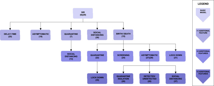
As mentioned above, compartmental models can be extended to consider further details. We have found models that incorporate the following features: asymptomatic individuals, births and deaths, delay-time, lock-down, quarantine, isolation, social distancing, and screening. Fig. 1 shows a classification of the SIR models reviewed in this article, and Table 1 lists them along with their equations. Multiple output choices have been considered in the study of the structural identifiability and observability of some models. In such cases the observations are listed in the Output column.

Fig. 1.

Classification of SIR models. Each block represents a model structure. The basic, three-compartment SIR model structure is on top of the tree. Every additional block is labelled with the additional feature that it contains with respect to its parent block. The darkness of the shade indicates the number of additional features with respect to the basic SIR model.

3.2. SEIR models

Individuals in the SEIR model are divided in four compartments: Susceptible (S), Exposed (E), Infected (I) and Recovered (R). Compared to the SIR models, the additional compartment $E$ allows for a more accurate description of diseases in which the incubation period and the latent period do not coincide, i.e. the period between which an infected becomes infectious. This is why SEIR models are in principle best suited to epidemics with a long incubation period such as COVID-19 (Franco, 2020).

Susceptible individuals move to the exposed class at a rate $\beta I\left(t\right)$, where $\beta$ is the transmission rate parameter. Exposed individuals become infected at rate $\kappa$, where $1∕\kappa$ is the average latent period. Infected individuals recover at rate $\gamma$, where $1∕\gamma$ is the average infectious period.

Thus, the set of differential equations describing the basic SEIR model is:

$$\dot{S}\left(t\right)=-\beta S\left(t\right)I\left(t\right)$$$$\dot{E}\left(t\right)=\beta S\left(t\right)I\left(t\right)-\kappa E\left(t\right)$$$$\dot{I}\left(t\right)=\kappa E\left(t\right)-\gamma I\left(t\right)$$$$\dot{R}\left(t\right)=\gamma I\left(t\right)$$ (7)

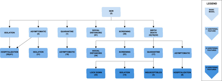
Existing extensions of SEIR models may incorporate some of the following features: asymptomatic individuals, births and deaths, hospitalization, quarantine, isolation, social distancing, screening and lock-down. Fig. 2 shows a classification of the models found in the literature; Table 2 lists them along with their equations.

Fig. 2.

Classification of SEIR models. Each block represents a model structure. The basic, four-compartment SEIR model structure is on top of the tree. Every additional block is labelled with the additional feature that it contains with respect to its parent block. The darkness of the shade indicates the number of additional features with respect to the basic SEIR model.

Table 2.

List of SEIR models and their main features.

ID	Ref.	States	Parameters	Output	ICS	Input	Equations
2	Roosa and Chowell (2019)	S, E, I, R	$\beta$, $\gamma$, k, K	$\begin{array}{cc}\hfill & \left(1\right)C\hfill \\ \hfill & \left(2\right)KC\hfill \end{array}$			$\begin{array}{cc}\hfill \dot{S}\left(t\right)& =-\beta SI∕N\hfill \\ \hfill \dot{E}\left(t\right)& =\beta SI∕N-kE\hfill \\ \hfill \dot{I}\left(t\right)& =kE-\gamma I\hfill \\ \hfill \dot{R}\left(t\right)& =\gamma I\hfill \\ \hfill \dot{C}\left(t\right)& =kE\hfill \end{array}$
34	Chitnis (2017)	S, E, I, R	$\beta$, $\gamma$, $\mu$, $ϵ$, r, K	KI			$\begin{array}{cc}\hfill \dot{S}\left(t\right)& =\Lambda -r\beta SI∕N-\mu S\hfill \\ \hfill \dot{E}\left(t\right)& =\beta SI∕N-ϵE-\mu E\hfill \\ \hfill \dot{I}\left(t\right)& =ϵE-\gamma I-\mu I\hfill \\ \hfill \dot{R}\left(t\right)& =\gamma I-\mu R\hfill \end{array}$
16	Roda et al. (2020)	S, E, I, R	$\beta$, $\rho$, $\mu$, d, $ϵ$, $\tau$, $E_0$, $I_0$	$\begin{array}{cc}\hfill & \left(1\right)\rho I+\tau \hfill \\ \hfill & \left(2\right)\mu I\hfill \end{array}$	$\begin{array}{cc}\hfill & S_0\hfill \\ \hfill & E_0\hfill \\ \hfill & I_0\hfill \\ \hfill & R_0\hfill \end{array}$		$\begin{array}{cc}\hfill \dot{S}\left(t\right)& =-\beta SI\hfill \\ \hfill \dot{E}\left(t\right)& =\beta SI-ϵE\hfill \\ \hfill \dot{I}\left(t\right)& =ϵE-(\rho +\mu )I\hfill \\ \hfill \dot{R}\left(t\right)& =\rho I-dR\hfill \end{array}$
51	McGee (2020)	S, E, I, De, Di, R, F	q, ${\mu }_i$, ${\mu }_d$, $\sigma$, ${\sigma }_d$, ${\theta }_e$, ${\theta }_i$, $\gamma$, ${\gamma }_d$, $\beta$, ${\beta }_d$, ${\varphi }_i$, ${\varphi }_e$, ${\mu }_0$	$\begin{array}{cc}\hfill & \left(1\right)De,Di,F\hfill \\ \hfill & \left(2\right)Di,F\hfill \end{array}$			$\begin{array}{cc}\hfill \dot{S}\left(t\right)& =-\beta SI∕N-q{\beta }_{d}SDi∕N+\nu N-{\mu }_{0}S\hfill \\ \hfill \dot{E}\left(t\right)& =\beta SI∕N+q{\beta }_{d}SDi∕N-\sigma E-{\theta }_e{\varphi }_{e}E-{\mu }_{0}E\hfill \\ \hfill \dot{I}\left(t\right)& =\sigma E-\gamma I-{\mu }_{i}I-{\theta }_i{\varphi }_{i}I-{\mu }_{0}I\hfill \\ \hfill \dot{De}\left(t\right)& ={\theta }_e{\varphi }_{e}E-{\sigma }_{d}De-{\mu }_{0}De\hfill \\ \hfill \dot{Di}\left(t\right)& ={\theta }_i{\varphi }_{i}I+{\sigma }_{d}De-{\gamma }_{d}Di-{\mu }_{d}Di-{\mu }_{0}Di\hfill \\ \hfill \dot{R}\left(t\right)& =\gamma I+{\gamma }_{d}Di-{\mu }_{0}R\hfill \\ \hfill \dot{F}\left(t\right)& ={\mu }_{i}I+{\mu }_{d}Di\hfill \end{array}$
14	Lopez and Rodo (2020)	S, E, I, Q, R, D, C	$\beta$, $\alpha$, $\gamma$, $\delta$, $\tau$	C, Q, D		k(t), $\lambda \left(t\right)$	$\begin{array}{cc}\hfill \dot{S}\left(t\right)& =\mu N-\alpha S-\beta SIN-\mu S\hfill \\ \hfill \dot{E}\left(t\right)& =\beta SIN-\mu E-\gamma E\hfill \\ \hfill \dot{I}\left(t\right)& =\gamma E-\delta I-\mu I\mu S\hfill \\ \hfill \dot{Q}\left(t\right)& =\delta I-\lambda Q-kQ-\mu Q\hfill \\ \hfill \dot{R}\left(t\right)& =\lambda Q-\mu S\hfill \\ \hfill \dot{D}\left(t\right)& =kQ\hfill \\ \hfill \dot{C}\left(t\right)& =\alpha S-\mu C-\tau C\hfill \end{array}$
61	Hubbs (2020)	S, E, I, R	p, $\alpha$, $\beta$, $\gamma$, K	KI			$\begin{array}{cc}\hfill \dot{S}\left(t\right)& =-p\beta SI\hfill \\ \hfill \dot{E}\left(t\right)& =p\beta SI-\alpha E\hfill \\ \hfill \dot{I}\left(t\right)& =\alpha E-\gamma I\hfill \\ \hfill \dot{R}\left(t\right)& =\gamma I\hfill \end{array}$
5	Pribylova and Hajnova (2020)	S, E, I, R, A	${\mu }_1$, ${\mu }_2$, $\gamma$, $\beta$, p	I			$\begin{array}{cc}\hfill \dot{S}\left(t\right)& =-\beta S(I+A)\hfill \\ \hfill \dot{E}\left(t\right)& =\beta S(I+A)-\gamma E\hfill \\ \hfill \dot{I}\left(t\right)& =\gamma pE-{\mu }_{1}I\hfill \\ \hfill \dot{A}\left(t\right)& =\gamma (1-p)E-{\mu }_{2}A\hfill \\ \hfill \dot{R}\left(t\right)& ={\mu }_{1}I+{\mu }_{2}A\hfill \end{array}$
1	Zha et al. (2020)	S, E, I, R, Q	$\varphi$, $\beta$, $\gamma$, w	Q			$\begin{array}{cc}\hfill \dot{S}\left(t\right)& =-\beta SI\hfill \\ \hfill \dot{E}\left(t\right)& =\beta SI-wE\hfill \\ \hfill \dot{I}\left(t\right)& =wE-\varphi I-(1-\varphi )\gamma I\hfill \\ \hfill \dot{R}\left(t\right)& =\gamma Q+(1-\varphi )\gamma I\hfill \\ \hfill \dot{Q}\left(t\right)& =-\gamma Q+\varphi I\hfill \end{array}$
3	Liangrong et al. (2020)	S, E, I, R Q, D, P	$\alpha$, $\beta$, $\gamma$, $\delta$ $E_0$, $I_0$	Q, R, D	$\begin{array}{cc}\hfill & S_0\hfill \\ \hfill & E_0\hfill \\ \hfill & I_0\hfill \\ \hfill & Q_0\hfill \\ \hfill & R_0\hfill \\ \hfill & D_0\hfill \\ \hfill & P_0\hfill \end{array}$	$\lambda \left(t\right)$, $\kappa \left(t\right)$	$\begin{array}{cc}\hfill \dot{S}\left(t\right)& =-\beta SI∕N-\alpha S\hfill \\ \hfill \dot{E}\left(t\right)& =\beta SI∕N-\gamma E\hfill \\ \hfill \dot{I}\left(t\right)& =\gamma E-\delta I\hfill \\ \hfill \dot{Q}\left(t\right)& =\delta I-\lambda Q-\kappa Q\hfill \\ \hfill \dot{R}\left(t\right)& =\lambda Q\hfill \\ \hfill \dot{D}\left(t\right)& =\kappa Q\hfill \\ \hfill \dot{P}\left(t\right)& =\alpha S\hfill \\ \hfill \end{array}$
4	Sameni (2020)	S, E, I, R, P	${\alpha }_e$, ${\alpha }_i$, $\rho$, $\beta$, $\mu$, $\kappa$, $e_0$	$\begin{array}{cc}\hfill & \left(1\right)S+vs\left(t\right)\hfill \\ \hfill & \left(1\right)I+vi\left(t\right)\hfill \\ \hfill & \left(1\right)R+vr\left(t\right)\hfill \\ \hfill & \left(1\right)P+vp\left(t\right)\hfill \\ \hfill & \left(2\right)P\hfill \end{array}$	$\begin{array}{cc}\hfill & N-e_0\hfill \\ \hfill & e_0\hfill \\ \hfill & 0\hfill \\ \hfill & 0\hfill \\ \hfill & 0\hfill \end{array}$	$\begin{array}{cc}\hfill & vs\left(t\right)\hfill \\ \hfill & vi\left(t\right)\hfill \\ \hfill & vr\left(t\right)\hfill \\ \hfill & vp\left(t\right)\hfill \end{array}$	$\begin{array}{cc}\hfill \dot{S}\left(t\right)& =-{\alpha }_{e}SE-{\alpha }_{i}SI\hfill \\ \hfill \dot{E}\left(t\right)& ={\alpha }_{e}SE+{\alpha }_{i}SI-\kappa E-\rho E\hfill \\ \hfill \dot{I}\left(t\right)& =\kappa E-\beta I-\mu I\hfill \\ \hfill \dot{R}\left(t\right)& =\beta I+\rho E\hfill \\ \hfill \dot{P}\left(t\right)& =\mu I\hfill \end{array}$
8	Eikenberry et al. (2020)	S, E, I, R A, H, D	$\delta$, $\alpha$, $\eta$, $\sigma$, ${\gamma }_a$, ${\gamma }_i$, ${\gamma }_h$ $\Phi$, $E_0$, $R_0$, $A_0$ $H_0$, $D_0$	D, H, I	$\begin{array}{cc}\hfill & 1e6\hfill \\ \hfill & E_0\hfill \\ \hfill & 50\hfill \\ \hfill & A_0\hfill \\ \hfill & H_0\hfill \\ \hfill & R_0\hfill \\ \hfill & D_0\hfill \end{array}$	$\beta \left(t\right)$	$\begin{array}{cc}\hfill \dot{S}\left(t\right)& =-\beta (I+\eta A)S∕N\hfill \\ \hfill \dot{E}\left(t\right)& =\beta (I+\eta A)S∕N-\sigma E\hfill \\ \hfill \dot{I}\left(t\right)& =\alpha \sigma E-\Phi I-{\gamma }_{i}I\hfill \\ \hfill \dot{A}\left(t\right)& =(1-\alpha )\sigma E-{\gamma }_{a}A\hfill \\ \hfill \dot{H}\left(t\right)& =\Phi I-\delta H-{\gamma }_{h}H\hfill \\ \hfill \dot{R}\left(t\right)& ={\gamma }_{i}I+{\gamma }_{a}A+{\gamma }_{h}H\hfill \\ \hfill \dot{D}\left(t\right)& =\delta H\hfill \end{array}$
38	Shi et al. (2020)	S, E, I, Sq, Eq, H, R	c, q, $\lambda$, $\beta$ ${\delta }_i$, ${\delta }_q$, $\alpha$, ${\gamma }_i$ ${\gamma }_h$, $\theta$	$\begin{array}{cc}\hfill & \left(1\right)I,R\hfill \\ \hfill & \left(2\right)H,viI,vrR\hfill \\ \hfill & \left(3\right)Sq,Eq\hfill \end{array}$		$\sigma \left(t\right)$	$\begin{array}{cc}\hfill \dot{S}\left(t\right)& =-(c\beta +cq(1-\beta ))S(I+\theta E)+\lambda Sq\hfill \\ \hfill \dot{E}\left(t\right)& =c\beta (1-q)S(I+\theta E)-\sigma E\hfill \\ \hfill \dot{I}\left(t\right)& =\sigma E-({\delta }_i+\alpha +{\gamma }_i)I\hfill \\ \hfill \dot{Sq}\left(t\right)& =cq(1-\beta )S(I+\theta E)-\lambda Sq\hfill \\ \hfill \dot{Eq}\left(t\right)& =cq\beta S(I+\theta E)-{\delta }_{q}Eq\hfill \\ \hfill \dot{H}\left(t\right)& ={\delta }_{i}I+{\delta }_{q}Eq-(\alpha +{\gamma }_h)H\hfill \\ \hfill \dot{R}\left(t\right)& ={\gamma }_{i}I+{\gamma }_{h}H\hfill \end{array}$
41	Roosa and Chowell (2019)	S, E, A, I, J, R, C	$\beta$, k, ${\gamma }_1$ ${\gamma }_2$, $\alpha$, $\rho$, q	$\begin{array}{cc}\hfill & \left(1\right)C\hfill \\ \hfill & \left(2\right)J,I\hfill \end{array}$			$\begin{array}{cc}\hfill \dot{S}\left(t\right)& =-\beta S(I+J+qA)∕N\hfill \\ \hfill \dot{E}\left(t\right)& =\beta S(I+J+qA)∕N-kE\hfill \\ \hfill \dot{A}\left(t\right)& =k(1-\rho )E-{\gamma }_{1}A\hfill \\ \hfill \dot{I}\left(t\right)& =k\rho E-(\alpha +{\gamma }_1)I\hfill \\ \hfill \dot{J}\left(t\right)& =\alpha I-{\gamma }_{2}J\hfill \\ \hfill \dot{R}\left(t\right)& ={\gamma }_1(A+I)+{\gamma }_{2}J\hfill \\ \hfill \dot{C}\left(t\right)& =\alpha I\hfill \end{array}$
39	McGee (2020)	S, E, I, De, Di, R, F	q, ${\mu }_i$, ${\mu }_d$, $\sigma$, ${\sigma }_d$, ${\theta }_e$, ${\theta }_i$, $\gamma$, ${\gamma }_d$, $\beta$, ${\beta }_d$, ${\varphi }_i$, ${\varphi }_e$	$\begin{array}{cc}\hfill & \left(1\right)F,Di\hfill \\ \hfill & \left(2\right)F,De,Di\hfill \end{array}$			$\begin{array}{cc}\hfill \dot{S}\left(t\right)& =-\beta SI∕N-q{\beta }_{d}SDi∕N\hfill \\ \hfill \dot{E}\left(t\right)& =\beta SI∕N+q{\beta }_{d}SDi∕N-\sigma E-{\theta }_e{\varphi }_{e}E\hfill \\ \hfill \dot{I}\left(t\right)& =\sigma E-\gamma I-{\mu }_{i}I-{\theta }_i{\varphi }_{i}I\hfill \\ \hfill \dot{De}\left(t\right)& ={\theta }_e{\varphi }_{e}E-{\sigma }_{d}De\hfill \\ \hfill \dot{Di}\left(t\right)& ={\theta }_i{\varphi }_{i}I+{\sigma }_{d}De-{\gamma }_{d}Di-{\mu }_{d}Di\hfill \\ \hfill \dot{R}\left(t\right)& =\gamma I+{\gamma }_{d}Di\hfill \\ \hfill \dot{F}\left(t\right)& ={\mu }_{i}I+{\mu }_{d}Di\hfill \end{array}$
17	Chatterjee et al. (2020)	S, E, I, R, Q, D	$\beta$, $ϵ$, $\gamma$, d, q, qt	$\begin{array}{cc}\hfill & \left(1\right)D\hfill \\ \hfill & \left(2\right)Q,D\hfill \\ \hfill & \left(3\right)D,I,Q\hfill \end{array}$	$\begin{array}{cc}\hfill & 249\hfill \\ \hfill & E_0\hfill \\ \hfill & q{Q}_0\hfill \\ \hfill & Q_0\hfill \\ \hfill & 23\hfill \\ \hfill & 5\hfill \end{array}$		$\begin{array}{cc}\hfill \dot{S}\left(t\right)& =-\beta SI\hfill \\ \hfill \dot{E}\left(t\right)& =\beta SI-ϵE\hfill \\ \hfill \dot{I}\left(t\right)& =ϵE-\gamma I-dI-qI\hfill \\ \hfill \dot{Q}\left(t\right)& =qI-qtQ-dQ\hfill \\ \hfill \dot{R}\left(t\right)& =\gamma I+qtQ\hfill \\ \hfill \dot{D}\left(t\right)& =dI+dQ\hfill \end{array}$
18	Jia et al. (2020)	S, E, I, A, R, Q, D	$\beta$, $\theta$, $\lambda$, $\sigma$, $\rho$, ${ϵ}_a$, ${ϵ}_i$, ${\gamma }_i$, ${\gamma }_a$, ${\gamma }_d$, p, $d_i$, $d_d$	$\begin{array}{cc}\hfill & \left(1\right)D,I,Q\hfill \\ \hfill & \left(2\right)Q,D\hfill \\ \hfill & \left(3\right)D\hfill \end{array}$	$\begin{array}{cc}\hfill & 9219849e3\hfill \\ \hfill & 4142251e2\hfill \\ \hfill & 3207\hfill \\ \hfill & 595\hfill \\ \hfill & 563\hfill \\ \hfill & 227\hfill \\ \hfill & 3\hfill \end{array}$		$\begin{array}{cc}\hfill \dot{S}\left(t\right)& =-\beta S(I+\theta A)-pS+\lambda Q\hfill \\ \hfill \dot{Q}\left(t\right)& =pS-\lambda Q\hfill \\ \hfill \dot{E}\left(t\right)& =\beta S(I+\theta A)-\sigma E\hfill \\ \hfill \dot{A}\left(t\right)& =\sigma (1-\rho )E-{ϵ}_{a}A-{\gamma }_{a}A\hfill \\ \hfill \dot{I}\left(t\right)& =\sigma \rho E-{\gamma }_{i}I-d_{i}I-{ϵ}_{i}I\hfill \\ \hfill \dot{D}\left(t\right)& ={ϵ}_{a}A+{ϵ}_{i}I-d_{d}D-{\gamma }_{d}D\hfill \\ \hfill \dot{R}\left(t\right)& ={\gamma }_{a}A+{\gamma }_{i}I+{\gamma }_{d}D\hfill \end{array}$
31	Dohare (2020)	S, E, I, A, J, R	$\alpha$, $\sigma$, h, r, q, f, ${\beta }_1$, ${\beta }_2$, $\varphi$, $\gamma$, $I_0$	$\begin{array}{cc}\hfill & \left(1\right)I,J\hfill \\ \hfill & \left(2\right)I\hfill \end{array}$	$\begin{array}{cc}\hfill & 0.9N\hfill \\ \hfill & 9(I_0+A_0)\hfill \\ \hfill & I_0\hfill \\ \hfill & I_{0}f\hfill \\ \hfill & 0\hfill \\ \hfill & 0\hfill \end{array}$		$\begin{array}{cc}\hfill \dot{S}\left(t\right)& =-\alpha \frac{E+I+A}{N}S-\sigma S\hfill \\ \hfill \dot{E}\left(t\right)& =\alpha \frac{E+I+A}{N}S-{\beta }_{1}E\hfill \\ \hfill \dot{I}\left(t\right)& ={\beta }_{1}hE+{\beta }_{2}rA-\varphi qI-\gamma (1-q)I\hfill \\ \hfill \dot{A}\left(t\right)& ={\beta }_1(1-h)E-{\beta }_{2}rA-\gamma (1-r)A\hfill \\ \hfill \dot{J}\left(t\right)& =\varphi qI-\gamma J\hfill \\ \hfill \dot{R}\left(t\right)& =\gamma (1-q)I+\gamma (1-r)A+\gamma J\hfill \end{array}$
32	Rahman and Kuddus (2020)	S, L, I, R	w, $\beta$, $\alpha$, $\gamma$, $\mu$	wL			$\begin{array}{cc}\hfill \dot{S}\left(t\right)& =A-\frac{\beta SI}{1+\alpha I}-\mu S\hfill \\ \hfill \dot{L}\left(t\right)& =\frac{\beta SI}{1+\alpha I}-(w+\mu )L\hfill \\ \hfill \dot{I}\left(t\right)& =wL-(\gamma +\mu )I\hfill \\ \hfill \dot{R}\left(t\right)& =\gamma I-\mu R\hfill \end{array}$
33	Fosu et al. (2020)	S, L, E, I, Q, R	$\gamma$, ${\beta }_1$, $\eta$, $\delta$, $\xi$, ${\theta }_2$, $ϵ$, ${\theta }_1$, ${\alpha }_1$, ${\alpha }_2$,	L, Q			$\begin{array}{cc}\hfill \dot{S}\left(t\right)& =\mu N-{\beta }_{1}SI-(\gamma +\eta )S+\delta L+\xi E\hfill \\ \hfill \dot{L}\left(t\right)& =\eta S-(\gamma +\delta )L\hfill \\ \hfill \dot{E}\left(t\right)& ={\beta }_{1}SI-(\gamma +{\theta }_2+ϵ+\xi )E\hfill \\ \hfill \dot{I}\left(t\right)& =ϵE-(\gamma +{\theta }_1+{\alpha }_2)I\hfill \\ \hfill \dot{Q}\left(t\right)& ={\theta }_{1}I+{\theta }_{2}E-(\gamma +{\alpha }_2)Q\hfill \\ \hfill \dot{R}\left(t\right)& ={\alpha }_{1}I+{\alpha }_{2}Q-\gamma R\hfill \end{array}$

4. Results and discussion

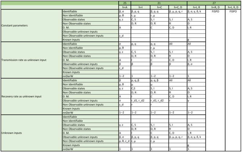
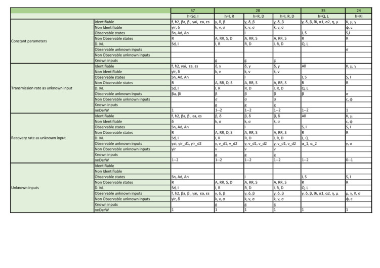
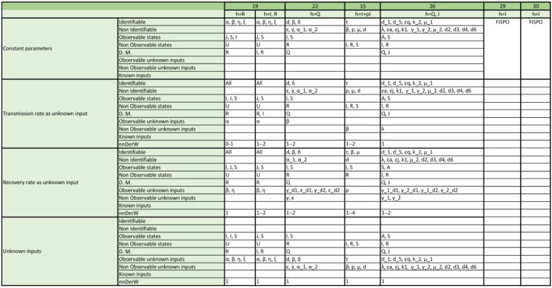
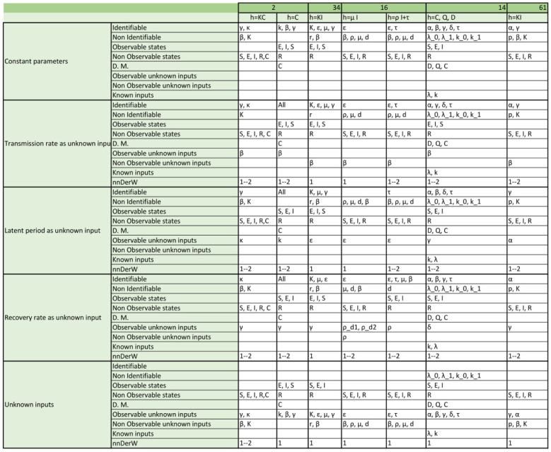
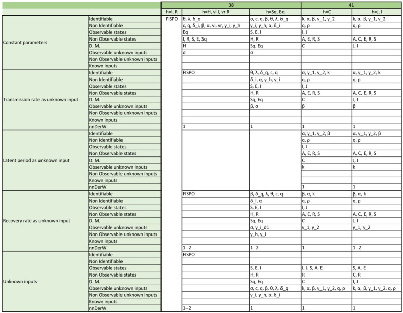
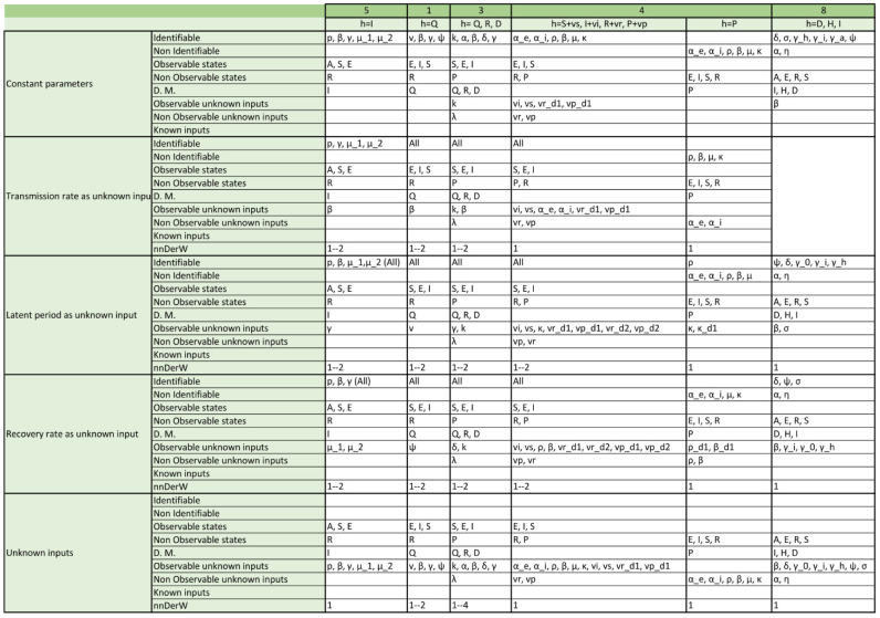
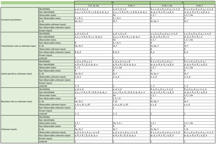
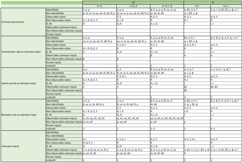
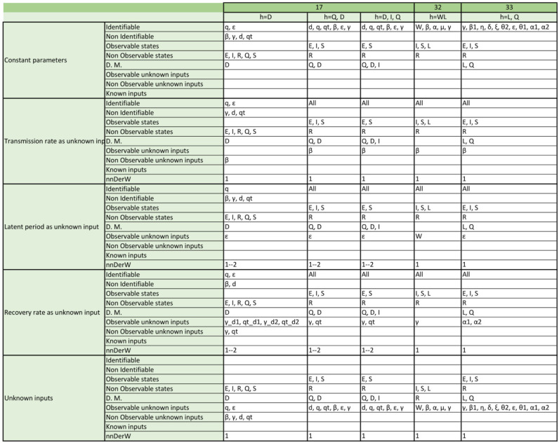
We analysed the structural identifiability and observability of the 17 SIR model structures (a total of 98 model versions considering the different output configurations and time-varying parameter assumptions) and 19 SEIR models (with a total of 157 model versions) listed in Table 1, Table 2. The detailed results for each model are given in Appendix, which reports the structural identifiability of each parame-ter and the observability of each state, for every model version. In the remainder of this section we provide an overview of the main results.

4.1. General patterns

The general patterns regarding state observability are as follows. The recovered state (R) is almost never observable unless it is directly measured (D.M.) as output; the only exceptions are two SEIR models, 31 and 38, for which R is observable under the assumption of time-varying parameters. The susceptible state (S), in contrast, is observable in roughly two thirds of the models (SIR: 65/98, SEIR: 103/157); this is also true for the exposed state (E) in the SEIR models. The infected state (I) is included in most studies among the outputs, either directly (D.M.) or indirectly measured (as part of a parameterized measurement function). When it is not considered in this way, its observability is generally similar to that of S (in 18/157 model versions I is not an output and it is observable in 13/18).

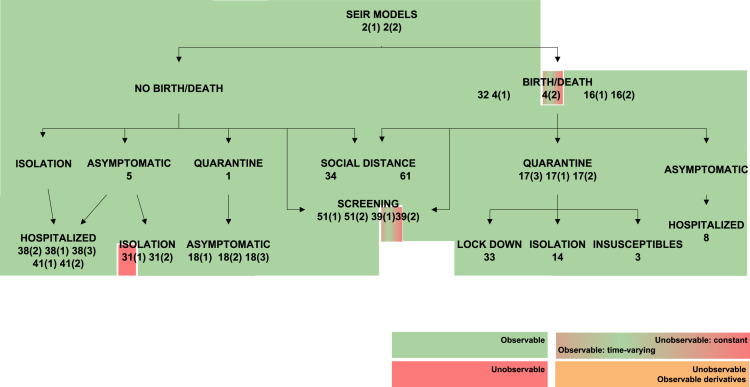
The transmission and recovery rates ($\beta$, $\gamma$) are the two parameters common to all SIR models. The transmission rate is identifiable in 59/98 model versions, and $\gamma$ in 51/98 and its derivatives in 12/98. SEIR models have a third parameter in common, the latent period ($\kappa$). It is identifiable in most of the models (145/157), as well as the recovery rate (111/157). The transmission rate is identifiable in 101/157 model versions, but it is not identifiable in any SEIR model version that accounts for social distancing (numbers 34 and 61); we found no clear pattern in the other models.

4.2. The effect of time-varying parameters

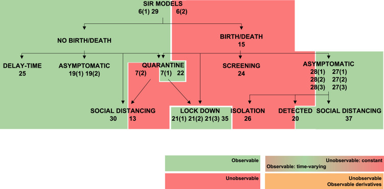
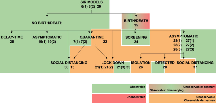
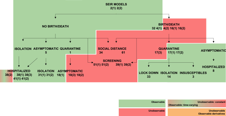
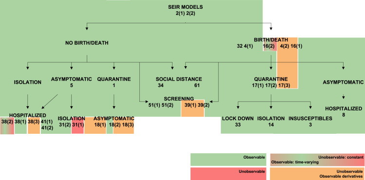
The transmission rate $\beta$, the recovery rate $\gamma$, and in SEIR models the latent period $\kappa$, can vary during an epidemic as a result of changes in the population’s behaviour (Chen et al., 2020, Liangrong et al., 2020), the introduction of new drugs or new medical equipment (Liangrong et al., 2020), or the reduction of the period duration as a result of high temperatures (Li & Zhao, 2019). To account for such variations, the present study has considered both the constant and the time-varying cases, by including the corresponding variables either in the constant parameter vector $\theta$ or in the unknown input vector $w\left(t\right)$, respectively, as described in Remark 1. Changing a parameter from constant to time-varying naturally influences structural identifiability and observability. This effect is graphically summarized in Fig. 3, Fig. 4, Fig. 5, Fig. 6, Fig. 7, which represent classes of models in tree form and classify them according to their observability. Each model is shaded with a colour, according to the observability of the parameter studied. Some models include different rates for different population groups: for example, they may consider two different transmission rates for symptomatic and asymptomatic individuals. For those models, each rate may have different observability properties when considered time-varying parameters; in such cases the model is depicted between two colour blocks (see for example the SIR 20 model in Fig. 3).

Fig. 3.

Observability of $\beta$ (transmission rate) in SIR models. Models in which $\beta$ is observable are shown in green, and non-observable in red. (For interpretation of the references to colour in this figure legend, the reader is referred to the web version of this article.)

Fig. 4.

Observability of $\gamma$ (recovery rate) in SIR models. Models in which $\gamma$ is observable are shown in green. Models in which it is unobservable if constant and observable if time-varying are shown in a green–red gradient. Finally, models in which only its time-derivatives are observable are shown in orange. (For interpretation of the references to colour in this figure legend, the reader is referred to the web version of this article.)

Fig. 5.

Observability of $\beta$ (transmission rate) in SEIR models. Models in which $\beta$ is observable are shown in green, and non-observable in red. Models in which it is unobservable if constant and observable if time-varying are shown in a green–red gradient. (For interpretation of the references to colour in this figure legend, the reader is referred to the web version of this article.)

Fig. 6.

Observability of $\kappa$ (latent period) in SEIR models. Models in which $\kappa$ is observable are shown in green, and non-observable in red. Models in which it is unobservable if constant and observable if time-varying are shown in a green–red gradient. (For interpretation of the references to colour in this figure legend, the reader is referred to the web version of this article.)

Fig. 7.

Observability of $\gamma$ (recovery rate) in SEIR models. Models in which $\gamma$ is observable are shown in green, and non-observable in red. Models in which it is unobservable if constant and observable if time-varying are shown in a green–red gradient. Finally, models in which only its time-derivatives are observable are shown in orange. (For interpretation of the references to colour in this figure legend, the reader is referred to the web version of this article.)

Changing $\beta$ from a constant to a time-varying parameter (or equivalently an unknown input) does not change its observability nor that of the other variables in SIR models. In contrast, this is not the case with the recovery rate $\gamma$, for which a somewhat counter-intuitive result may be obtained: by changing $\gamma$ from a constant to a continuous function of time with at least a non-zero derivative, its model can become more observable and identifiable — despite the fact that it is an unknown function. An example of this is the SIR model 15: if $\gamma$ is constant the model has only one identifiable parameter, $\tau$, and no observable states; if $\gamma$ is time-varying with at least one non-zero derivative, two parameters become identifiable ($\beta$, $\mu$), two states become observable (I, S), and $\gamma$ itself is observable. In the other models, when $\gamma$ is not identifiable as a constant nor observable as an unknown input, its successive derivatives are observable.

For the SEIR models, the consideration of the $\beta$ parameter as an unknown input function follows a similar trend to that of the SIR models with the exception of model 38, which gains both observability and identifiability and becomes FISPO. Considering the recovery rate $\gamma$ (Fig. 7) or the latent period $\kappa$ (Fig. 6) individually as time-varying parameters generally leads to greater observability, except for model 31(1). As an example, in model 39(2) one of the unknown inputs becomes observable, three states become observable (S, E, I), and three parameters become identifiable ($\gamma$, ${\mu }_i$, $\beta$); or the 16(2) model, in which both its input and three states (S, E, I) become observable and two parameters ($\mu$, $\beta$) become identifiable.

Besides the transmission rate, latent period, and recovery rate, other rates (screening, disease-related deaths, and isolation) have also been considered as time-varying parameters in some studies. The observability of most models is not modified if these parameters are allowed to change in time; the exception being 8 models which gain observability. An example is the SEIR model 41(1), which has seven parameters, seven states, and one output. Assuming constant parameters, five of them are structurally identifiable ($\kappa$, $\alpha$, $\beta$, ${\gamma }_1$, ${\gamma }_2$) and two are unidentifiable (q, $\rho$), while there are three observable states (I, J, C) and four unobservable states (S, E, A, R) (Roosa & Chowell, 2019). However, when the parameter $\rho$ (which describes the proportion of exposed/latent individuals who become clinically infectious) is considered time-varying, all parameters become identifiable (including $\rho$) and six states become observable (all except R, which is never observable unless it can be directly measured, as we have already mentioned).

The fact that allowing an unknown quantity to change in time can improve its observability – and also the observability of other variables in a model – may seem paradoxical. An intuitive explanation can be obtained from the study of the symmetry in the model structure. The existence of Lie symmetries amounts to the possibility of transforming parameters and state variables while leaving the output unchanged, i.e. their existence amounts to lack of structural identifiability and/or observability (Yates, Evans, & Chappell, 2009). The STRIKE-GOLDD toolbox used in this paper includes procedures for finding Lie symmetries (Massonis & F. Villaverde, 2020). Let us use the SIR 15 model as an example. This model has five parameters ($\tau$, $\beta$, $\rho$, $\mu$, d), of which only $\tau$ is identifiable if assumed constant. The model contains the following symmetry:

$${\mu }^{\ast }=\mu +ϵ\rho ,$$

where $ϵ$ is the parameter of the Lie group of transformations. Thus, there is a symmetry between $\rho$ and $\mu$ that makes them unidentifiable: changes in one parameter can be compensated by changes in the other one. However, if $\rho$ is time-varying and $\mu$ is constant, the latter cannot compensate the changes of the former, and the symmetry is broken. Indeed, if $\rho$ is considered time-varying the model gains identifiability (not only $\mu$, but also $\tau$ and $\beta$ become identifiable) and observability (S, I and $\rho$ become observable).

4.3. Applying the results in practice: an illustrative example

Let us now illustrate how the results of this study may be applied in a realistic scenario. We use as an example the model SIR 26, which has 6 states (S, I, R, A, Q, J) and 16 parameters ($d_1$, $d_2$, $d_3$, $d_4$, $d_5$, $d_6$, $k_1$, $k_2$, $\lambda$, ${\gamma }_1$, ${\gamma }_2$, ${ϵ}_a$, ${ϵ}_q$, ${ϵ}_j$, ${\mu }_1$, ${\mu }_2$); its equations are shown in Table 1. This model includes the following additional features with respect to the basic SIR model: birth/death, asymptomatic individuals (A), quarantine (Q), and isolation (J). In its original publication two states were measured (Q, J). With these two states as outputs the model has five identifiable parameters ($d_1$, $d_5$, ${ϵ}_q$, $k_2$, ${\mu }_1$) and two observable states (A, I); thus, there are two unobservable states (S, R) and ten unidentifiable parameters.

If we are interested in estimating e.g. the number of susceptible individuals (S), this model would not be appropriate. How should we proceed in that scenario?

One way of improving observability could be by including more outputs (option 1). For example, since there is a separate class for asymptomatic individuals (A), the infected compartment (I) considers only individuals with symptoms, and we could assume that they can be detected. By including ‘I’ in the output set, the structural identifiability and observability of the model improves: six more parameters are identifiable ($\lambda$, ${ϵ}_a$, ${ϵ}_j$, $d_4$, $k_1$, ${\mu }_2$) and the state in which we are interested (S) becomes observable.

However, including more outputs is not always realistic. Another possibility would then be to reduce the complexity of the model by decreasing the number of additional features (option 2). For example, leaving out the asymptomatic compartment leads to the following model:

$$\dot{S\left(t\right)}=bN-S(I\lambda +\lambda {ϵ}_{q}Q+\lambda {ϵ}_{j}J+d_1)$$

$$\dot{I\left(t\right)}=S(I\lambda +\lambda {ϵ}_{q}Q+\lambda {ϵ}_{j}J)-({\gamma }_1+{\mu }_1+{\mu }_2+d_2)I$$

$$\dot{R\left(t\right)}={\gamma }_{1}I+{\gamma }_{2}J-d_{3}R$$

$$\dot{Q\left(t\right)}={\mu }_{1}I-(k_2+d_5)Q$$

$$\dot{J\left(t\right)}=k_{2}Q+{\mu }_{2}I-({\gamma }_2+d_6)J$$

The output of the model is the same, Q, J. In this case, the model has eight identifiable parameters ($\lambda$, ${ϵ}_q$, ${ϵ}_j$, $d_1$, $d_5$, ${\mu }_1$, ${\mu }_2$, $k_2$) and two observable states (S, I).

A third possibility is to simplify the parameterization of the model (option 3). This model considers a different death rate for every compartment ($d_i,i=1,\dots ,6$.). With some loss of generality, we could consider a specific death rate for infected individuals, $d_I=d_2$, and a general death rate $d$ for all non-infected and asymptomatic individuals, $d=d_1=d_3=d_4=d_5=d_6$. This reduction of the number of parameters leads to a better observability to the model: the only unidentifiable parameters are $d_2,{\gamma }_1$, and $k_1$, and the only non-observable state is R. Thus, this option also allows to identify S.

Finally, a fourth possible course of action is to reparameterize the model using identifiable combinations. This solution entails reducing the number of parameters involved in the model, with new variables consisting of e.g. the product or quotient of some parameters and/or states. These new variables are identifiable (observable) combinations, although the individual variables are not independently identifiable nor observable. There are several methods for finding identifiable combinations, with theoretical bases including Taylor series (Evans & Chappell, 2000), Lie Algebra (Massonis and F. Villaverde, 2020, Merkt et al., 2015, Sedoglavic, 2002), Gröbner bases (Meshkat et al., 2014), and bootstrap (Hengl, Kreutz, Timmer, & Maiwald, 2007). These methods can be used to find functionally related parameters and/or identifiable combinations of them. This information provides hints for generating identifiable model reparameterizations, although this step requires some user intervention. As an example, consider the simplest SIR model 6, in which the parameter combination $\beta ∕K$ is identifiable. Reparameterizing the model in this way makes it identifiable, although it is still impossible to estimate either the transmission rate or the ratio of reported cases. In addition, the three states would also have to be scaled by one of the above-mentioned parameters, thus losing their original meaning.

5. Conclusions

Our analyses have shown that a fraction of the models found in the literature have unidentifiable parameters. Key parameters such as the transmission rate ($\beta$), the recovery rate ($\gamma$), and the latent period ($\kappa$) are structurally identifiable in most, but not all, models. The transmission and recovery rates are identifiable in roughly two thirds of the models, and the latent period in almost all ($>90\text{\%}$) of them. Likewise, the states corresponding to the number of susceptible (S) and exposed (E) individuals are non-observable in roughly one third of the model versions analysed in this paper. The number of infected individuals (I) can usually be directly measured, but it is non-observable in one third of the model versions in which it is not measured. The situation is worse for the number of recovered individuals (R), which is almost never observable unless it is directly measured. Many models include other states in addition to S, E, I, and R, which are not always observable either.

The transmission rate and other parameters may vary during the course of an epidemic, as a result of a number of factors such as changes in public policy, population behaviour, or environmental conditions. To account for these variations, in the present study we have considered both the constant and the time-varying parameter case. Somewhat unexpectedly, we found that allowing for variability in an unknown parameter often improves the observability and/or identifiability of the model. This phenomenon might be explained by the contribution of this variability to the removal of symmetries in the model structure. Structural identifiability and observability depend on which states or functions are measured. The lack of these properties may in principle be surmounted by choosing the right set of outputs (Anguelova, Karlsson, & Jirstrand, 2012), but the required measurements are not always possible to perform in practice. Epidemiological models are a clear example of this; limitations such as lack of testing or the existence of asymptomatic individuals usually make it impossible to have measurements of all states. An alternative to measuring more states is to use a model with fewer compartments and/or a simpler parameterization, thus decreasing the number of states and/or parameters. Reducing the model dimension in this way may achieve observability and identifiability.

Even when it is not possible (or practical) to avoid non-observability or non-identifiability by any means, the model may still be useful, as long as it is only used to infer its observable states or identifiable parameters. For example, we may be interested in determining the transmission rate $\beta$ but not the number of recovered individuals R; in such case it is fine to use a model in which $\beta$ is identifiable even if R is not observable. Of course, this means that, to ensure that a model is properly used, it is necessary to characterize its identifiability and observability in detail, to know if the quantity of interest is observable/identifiable.

The contribution of this work has been to provide such a detailed analysis of the structural identifiability and observability of a large set of compartmental models of COVID-19 presented in the recent literature. The results of our analyses can be used to avoid the pitfalls caused by non-identifiability and non-observability. By classifying the existing models according to these properties, and arranging them in a structured way as a function of the compartments that they include, our study has answered the following question: given the sets of existing models and available measurements, which model is appropriate for inferring the value of some particular parameters, and/or to predict the time course of the states of interest?

Declaration of Competing Interest

The authors declare that they have no known competing financial interests or personal relationships that could have appeared to influence the work reported in this paper.

Appendix. Detailed structural identifiability and observability results

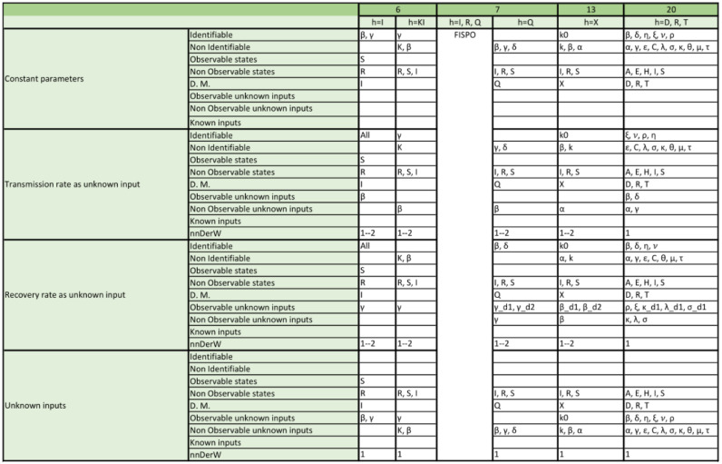
The tables included in the following pages report the results of the observability and structural identifiability analyses of all the model variants considered in this paper. Each block of rows represents one of the following assumptions:

• •All parameters considered constant (i.e. as is usually the case in the original publications).
• •Transmission rate $\beta$ considered time-varying.
• •Latent period $\kappa$ considered time-varying (only in SEIR models; SIR models do not have this parameter).
• •Recovery rate $\gamma$ considered time-varying.
• •All parameters considered time-varying.

Within each block, each row provides detailed information about identifiable and non-identifiable parameters, observable and non-observable states, directly measured (D.M.) states, observable and unobservable unknown inputs (and time-varying parameters), known inputs, and number of derivatives of the unknown inputs (and time-varying parameters) assumed to be non-zero (nnDerW). The suffix $\text{\_}$ d number represents the $n^{th}$ derivative of an unknown function (e.g. $\beta \text{\_}d1$ is the first derivative of the time-varying parameter $\beta$).

The blank blocks in the tables of the SEIR models numbers 38 and 8 indicate that the corresponding time-varying case is already considered in the original formulation of the model. The SIR models 29 and 30 have only been studied in their original form, i.e. without considering time-varying parameters, because these models do not contain the common parameters of the SIR models; instead they use the $R_0$ constant.

References

- Acemoglu D., Chernozhukov V., Werning I., Whinston M.D. National Bureau of Economic Research; 2020. A multi-risk SIR model with optimally targeted lockdown. [Google Scholar]
- Adam D. Special report: The simulations driving the world’s response to COVID-19. Nature. 2020;580(7803):316. doi: 10.1038/d41586-020-01003-6. [DOI] [PubMed] [Google Scholar]
- Alahmadi A., Belet S., Black A., Cromer D., Flegg J.A., House T., et al. Influencing public health policy with data-informed mathematical models of infectious diseases: Recent developments and new challenges. Epidemics. 2020 doi: 10.1016/j.epidem.2020.100393. [DOI] [PubMed] [Google Scholar]
- Alvarez F.E., Argente D., Lippi F. National Bureau of Economic Research; 2020. A simple planning problem for COVID-19 lockdown. [Google Scholar]
- Anguelova M., Karlsson J., Jirstrand M. Minimal output sets for identifiability. Mathematical Biosciences. 2012;239(1):139–153. doi: 10.1016/j.mbs.2012.04.005. [DOI] [PubMed] [Google Scholar]
- Arriola L., Hyman J.M. Mathematical and statistical estimation approaches in epidemiology. Springer; 2009. Sensitivity analysis for uncertainty quantification in mathematical models; pp. 195–247. [Google Scholar]
- Brauer F. Mathematical epidemiology. Springer Berlin Heidelberg; Berlin, Heidelberg: 2008. Compartmental models in epidemiology; pp. 19–79. [Google Scholar]
- Springer Berlin Heidelberg; 2008. Mathematical epidemiology. [Google Scholar]
- Brouwer A.F., Meza R., Eisenberg M.C. Integrating measures of viral prevalence and seroprevalence: a mechanistic modelling approach to explaining cohort patterns of human papillomavirus in women in the USA. Philosophical Transactions of the Royal Society B. 2019;374(1773) doi: 10.1098/rstb.2018.0297. [DOI] [PMC free article] [PubMed] [Google Scholar]
- Casella F. 2020. Can the COVID-19 epidemic be controlled on the basis of daily test reports? arXiv preprint arXiv:2003.06967. [Google Scholar]
- Castro M., Ares S., Cuesta J.A., Manrubia S. 2020. Predictability: Can the turning point and end of an expanding epidemic be precisely forecast? arXiv:2004.08842. [DOI] [PMC free article] [PubMed] [Google Scholar]
- Chapman J.D., Evans N.D. The structural identifiability of susceptible-infective-recovered type epidemic models with incomplete immunity and birth targeted vaccination. Biomedical Signal Processing and Control. 2009;4(4):278–284. [Google Scholar]
- Chatterjee K., Chatterjee K., Kumar A., Shankar S. Healthcare impact of COVID-19 epidemic in India: A stochastic mathematical model. Medical Journal Armed Forces India. 2020;76(2):147–155. doi: 10.1016/j.mjafi.2020.03.022. [DOI] [PMC free article] [PubMed] [Google Scholar]
- Chen Y.-C., Lu P.-E., Chang C.-S., Liu T.-H. 2020. A time-dependent SIR model for COVID-19 with undetectable infected persons. arXiv:2003.00122. [DOI] [PMC free article] [PubMed] [Google Scholar]
- Chitnis, N. (2017). Introduction to SEIR models. In Workshop on mathematical models of climate variability,environmental change and infectious diseases, Trieste, Italy.
- Chowell G. Fitting dynamic models to epidemic outbreaks with quantified uncertainty: a primer for parameter uncertainty, identifiability, and forecasts. Infectious Disease Modelling. 2017;2(3):379–398. doi: 10.1016/j.idm.2017.08.001. [DOI] [PMC free article] [PubMed] [Google Scholar]
- Cobey S. Modeling infectious disease dynamics. Science. 2020;368(6492):713–714. doi: 10.1126/science.abb5659. [DOI] [PubMed] [Google Scholar]
- Currie C.S., Fowler J.W., Kotiadis K., Monks T., Onggo B.S., Robertson D.A., et al. How simulation modelling can help reduce the impact of COVID-19. Journal of Simulation. 2020:1–15. [Google Scholar]
- DiStefano III J. Academic Press; 2015. Dynamic systems biology modeling and simulation. [Google Scholar]
- Dohare R. Mathematical model of transmission dynamics with mitigation and health measures for SARS-CoV-2 infection in European countries. Research Square. 2020 [Google Scholar]
- Eikenberry S.E., Mancuso M., Iboi E., Phan T., Eikenberry K., Kuang Y., et al. To mask or not to mask: Modeling the potential for face mask use by the general public to curtail the COVID-19 pandemic. Infectious Disease Modelling. 2020;5:293–308. doi: 10.1016/j.idm.2020.04.001. [DOI] [PMC free article] [PubMed] [Google Scholar]
- Eisenberg M.C., Robertson S.L., Tien J.H. Identifiability and estimation of multiple transmission pathways in cholera and waterborne disease. Journal of Theoretical Biology. 2013;324:84–102. doi: 10.1016/j.jtbi.2012.12.021. [DOI] [PubMed] [Google Scholar]
- Evans N., Chapman M., Chappell M., Godfrey K. The structural identifiability of a general epidemic (SIR) model with seasonal forcing. IFAC Proceedings Volumes. 2002;35(1):109–114. [Google Scholar]
- Evans N.D., Chappell M.J. Extensions to a procedure for generating locally identifiable reparameterisations of unidentifiable systems. Mathematical Biosciences. 2000;168(2):137–159. doi: 10.1016/s0025-5564(00)00047-x. [DOI] [PubMed] [Google Scholar]
- Evans N.D., White L.J., Chapman M.J., Godfrey K.R., Chappell M.J. The structural identifiability of the susceptible infected recovered model with seasonal forcing. Mathematical Biosciences. 2005;194(2):175–197. doi: 10.1016/j.mbs.2004.10.011. [DOI] [PubMed] [Google Scholar]
- Faranda D., Castillo I.P., Hulme O., Jezequel A., Lamb J.S., Sato Y., et al. Asymptotic estimates of SARS-CoV-2 infection counts and their sensitivity to stochastic perturbation. Chaos. An Interdisciplinary Journal of Nonlinear Science. 2020;30(5) doi: 10.1063/5.0008834. [DOI] [PMC free article] [PubMed] [Google Scholar]
- Fosu G., Opong J., Appati J. Construction of compartmental models for COVID-19 with quarantine, lockdown and vaccine interventions. SSRN Electronic Journal. 2020 [Google Scholar]
- Franco E. 2020. A feedback SIR (fSIR) model highlights advantages and limitations of infection-based social distancing. arXiv:2004.13216. [Google Scholar]
- Gaeta G. 2020. A simple SIR model with a large set of asymptomatic infectives. arXiv:2003.08720. [Google Scholar]
- Gallina R. Universita degli studi di Padova; 2012. Dynamic models for the analysis of epidemic spreads. [Ph.D. thesis] [Google Scholar]
- Gevertz J., Greene J., Hixahuary Sanchez Tapia C., Sontag E.D. 2020. A novel COVID-19 epidemiological model with explicit susceptible and asymptomatic isolation compartments reveals unexpected consequences of timing social distancing. medRxiv, Cold Spring Harbor Laboratory Press. [DOI] [PMC free article] [PubMed] [Google Scholar]
- Giordano G., Blanchini F., Bruno R., Colaneri P., Di Filippo A., Di Matteo A., et al. Modelling the COVID-19 epidemic and implementation of population-wide interventions in Italy. Nature Medicine. 2020 doi: 10.1038/s41591-020-0883-7. [DOI] [PMC free article] [PubMed] [Google Scholar]
- Hengl S., Kreutz C., Timmer J., Maiwald T. Data-based identifiability analysis of non-linear dynamical models. Bioinformatics. 2007;23(19):2612–2618. doi: 10.1093/bioinformatics/btm382. [DOI] [PubMed] [Google Scholar]
- Hermann R., Krener A.J. Nonlinear controllability and observability. IEEE Transactions on Automatic Control. 1977;22(5):728–740. [Google Scholar]
- Hethcote H., Zhien M., Shengbing L. Effects of quarantine in six endemic models for infectious diseases. Mathematical Biosciences. 2002;180(1):141–160. doi: 10.1016/s0025-5564(02)00111-6. [DOI] [PubMed] [Google Scholar]
- Holmdahl I., Buckee C. Wrong but useful—what COVID-19 epidemiologic models can and cannot tell us. New England Journal of Medicine. 2020 doi: 10.1056/NEJMp2016822. [DOI] [PubMed] [Google Scholar]
- Hong H., Ovchinnikov A., Pogudin G., Yap C. SIAN: software for structural identifiability analysis of ode models. Bioinformatics. 2019;35(16):2873–2874. doi: 10.1093/bioinformatics/bty1069. [DOI] [PubMed] [Google Scholar]
- Hubbs C. 2020. Social distancing to slow the coronavirus. https://towardsdatascience.com/social-distancing-to-slow-the-coronavirus-768292f04296. [Google Scholar]
- Janzén D.L., Bergenholm L., Jirstrand M., Parkinson J., Yates J., Evans N.D., et al. Parameter identifiability of fundamental pharmacodynamic models. Frontiers in Physiology. 2016;7:590. doi: 10.3389/fphys.2016.00590. [DOI] [PMC free article] [PubMed] [Google Scholar]
- Jia J., Ding J., Liu S., Liao G., Li J., Duan B., et al. Modeling the control of COVID-19: impact of policy interventions and meteorological factors. Electronic Journal of Differential Equations. 2020;2020:1–24. [Google Scholar]
- Kao Y.-H., Eisenberg M.C. Practical unidentifiability of a simple vector-borne disease model: Implications for parameter estimation and intervention assessment. Epidemics. 2018;25:89–100. doi: 10.1016/j.epidem.2018.05.010. [DOI] [PMC free article] [PubMed] [Google Scholar]
- Karlsson, J., Anguelova, M., & Jirstrand, M. (2012). An efficient method for structural identiability analysis of large dynamic systems. In 16th IFAC symposium on system identification, vol. 16 (pp. 941–946).
- Kim M., Milner F. A mathematical model of epidemics with screening and variable infectivity. Mathematical and Computer Modelling. 1995;21(7):29–42. [Google Scholar]
- Köhler J., Schwenkel L., Koch A., Berberich J., Pauli P., Allgöwer F. 2020. Robust and optimal predictive control of the COVID-19 outbreak. arXiv preprint arXiv:2005.03580. [DOI] [PMC free article] [PubMed] [Google Scholar]
- Li M.Y. Springer; 2018. An introduction to mathematical modeling of infectious diseases, vol. 2. [Google Scholar]
- Li F., Zhao X.-Q. A periodic SEIRS epidemic model with a time-dependent latent period. Journal of Mathematical Biology. 2019;78 doi: 10.1007/s00285-018-1319-6. [DOI] [PubMed] [Google Scholar]
- Liangrong P., Yang W., Zhang D., Zhuge C., Hong L. 2020. Epidemic analysis of COVID-19 in China by dynamical modeling. arXiv:2002.06563. [Google Scholar]
- Ligon T.S., Fröhlich F., Chiş O.T., Banga J.R., Balsa-Canto E., Hasenauer J. Genssi 2.0: multi-experiment structural identifiability analysis of SBML models. Bioinformatics. 2018;34(8):1421–1423. doi: 10.1093/bioinformatics/btx735. [DOI] [PMC free article] [PubMed] [Google Scholar]
- Lofgren E.T., Halloran M.E., Rivers C.M., Drake J.M., Porco T.C., Lewis B., et al. Opinion: Mathematical models: A key tool for outbreak response. Proceedings of the National Academy of Sciences. 2014;111(51):18095–18096. doi: 10.1073/pnas.1421551111. [DOI] [PMC free article] [PubMed] [Google Scholar]
- Lopez L.R., Rodo X. 2020. A modified SEIR model to predict the COVID-19 outbreak in Spain and Italy: simulating control scenarios and multi-scale epidemics. Cold Spring Harbor Laboratory Press. [DOI] [PMC free article] [PubMed] [Google Scholar]
- Lourenco J., Paton R., Ghafari M., Kraemer M., Thompson C., Simmonds P., et al. 2020. Fundamental principles of epidemic spread highlight the immediate need for large-scale serological surveys to assess the stage of the SARS-CoV-2 epidemic. [Google Scholar]
- Maier B.F., Brockmann D. 2020. Effective containment explains subexponential growth in recent confirmed COVID-19 cases in China. 368 (6492) 742–746, American Association for the Advancement of Science. [DOI] [PMC free article] [PubMed] [Google Scholar]
- Martcheva M. Springer; 2015. An introduction to mathematical epidemiology, vol. 61. [Google Scholar]
- Massonis G., F. Villaverde A. Finding and breaking Lie symmetries: Implications for structural identifiability and observability in biological modelling. Symmetry. 2020;12:469. [Google Scholar]
- McGee R.S. GitHub repository. GitHub; 2020. Models of SEIRS epidemic dynamics with extensions, including network-structured populations, testing, contact tracing, and social distancing. https://https://github.com/ryansmcgee/seirsplus. [Google Scholar]
- Merkt B., Timmer J., Kaschek D. Higher-order Lie symmetries in identifiability and predictability analysis of dynamic models. Physical Review E. 2015;92(1) doi: 10.1103/PhysRevE.92.012920. [DOI] [PubMed] [Google Scholar]
- Meshkat N., Kuo C.E.-z., DiStefano III J. On finding and using identifiable parameter combinations in nonlinear dynamic systems biology models and COMBOS: A novel web implementation. PLoS One. 2014;9(10) doi: 10.1371/journal.pone.0110261. [DOI] [PMC free article] [PubMed] [Google Scholar]
- Prague M., Wittkop L., Clairon Q., Dutartre D., Thiebaut R., Hejblum B.P. 2020. Population modeling of early COVID-19 epidemic dynamics in french regions and estimation of the lockdown impact on infection rate. medRxiv. [Google Scholar]
- Pribylova L., Hajnova V. 2020. SEIAR model with asymptomatic cohort and consequences to efficiency of quarantine government measures in COVID-19 epidemic. arXiv:2004.02601. [Google Scholar]
- Rahman A., Kuddus M.A. 2020. Modelling the transmission dynamics of COVID-19 in six high burden countries. Cold Spring Harbor Laboratory Press. [DOI] [PMC free article] [PubMed] [Google Scholar]
- Raimúndez E., Dudkin E., Vanhoefer J., Alamoudi E., Merkt S., Fuhrmann L., et al. COVID-19 outbreak in wuhan demonstrates the limitations of publicly available case numbers for epidemiological modelling. medRxiv. 2020 doi: 10.1016/j.epidem.2021.100439. [DOI] [PMC free article] [PubMed] [Google Scholar]
- Roda W.C., Varughese M.B., Han D., Li M.Y. Why is it difficult to accurately predict the COVID-19 epidemic? Infectious Disease Modelling. 2020;5:271–281. doi: 10.1016/j.idm.2020.03.001. [DOI] [PMC free article] [PubMed] [Google Scholar]
- Roosa K., Chowell G. Assessing parameter identifiability in compartmental dynamic models using a computational approach: application to infectious disease transmission models. Theoretical Biology and Medical Modelling. 2019;16(1):1. doi: 10.1186/s12976-018-0097-6. [DOI] [PMC free article] [PubMed] [Google Scholar]
- Saccomani M., Bellu G., Audoly S., d’Angio L. International conference on computational methods in systems biology. Springer; 2019. A new version of DAISY to test structural identifiability of biological models; pp. 329–334. [Google Scholar]
- Sameni R. 2020. Mathematical modeling of epidemic diseases; a case study of the COVID-19 coronavirus. arXiv preprint arXiv:2003.11371. [Google Scholar]
- Scarpino S.V., Petri G. On the predictability of infectious disease outbreaks. Nature Communications. 2019;10(1):1–8. doi: 10.1038/s41467-019-08616-0. [DOI] [PMC free article] [PubMed] [Google Scholar]
- Sedoglavic A. A probabilistic algorithm to test local algebraic observability in polynomial time. Journal of Symbolic Computation. 2002;33:735–755. [Google Scholar]
- Shi P., Cao S., Feng P. 2020. SEIR transmission dynamics model of 2019 nCoV coronavirus with considering the weak infectious ability and changes in latency duration. Cold Spring Harbor Laboratory Press. [Google Scholar]
- Thomaseth K., Saccomani M.P. Local identifiability analysis of nonlinear ODE models: how to determine all candidate solutions. IFAC-PapersOnLine. 2018;51(2):529–534. [Google Scholar]
- Tunali E.T., Tarn T.-J. New results for identifiability of nonlinear systems. IEEE Transactions on Automatic Control. 1987;32(2):146–154. [Google Scholar]
- Tuncer N., Le T.T. Structural and practical identifiability analysis of outbreak models. Mathematical Biosciences. 2018;299:1–18. doi: 10.1016/j.mbs.2018.02.004. [DOI] [PubMed] [Google Scholar]
- Villaverde A.F. Observability and structural identifiability of nonlinear biological systems. Complexity. 2019;2019 [Google Scholar]
- Villaverde A.F., Barreiro A., Papachristodoulou A. Structural identifiability of dynamic systems biology models. PLoS Computational Biology. 2016;12(10) doi: 10.1371/journal.pcbi.1005153. [DOI] [PMC free article] [PubMed] [Google Scholar]
- Villaverde A.F., Tsiantis N., Banga J.R. Full observability and estimation of unknown inputs, states, and parameters of nonlinear biological models. Journal of the Royal Society Interface. 2019;16 doi: 10.1098/rsif.2019.0043. [DOI] [PMC free article] [PubMed] [Google Scholar]
- Yates J.W., Evans N.D., Chappell M.J. Structural identifiability analysis via symmetries of differential equations. Automatica. 2009;45(11):2585–2591. [Google Scholar]
- Zha W.-t., Pang F.-r., Zhou N., Wu B., Liu Y., Du Y.-b., et al. Research about the optimal strategies for prevention and control of varicella outbreak in a school in a central city of China: based on an SEIR dynamic model. Epidemiology and Infection. 2020;148 doi: 10.1017/S0950268819002188. [DOI] [PMC free article] [PubMed] [Google Scholar]
- Zheng W. 2020. Total variation regularization for compartmental epidemic models with time-varying dynamics. arXiv:2004.00412. [Google Scholar]