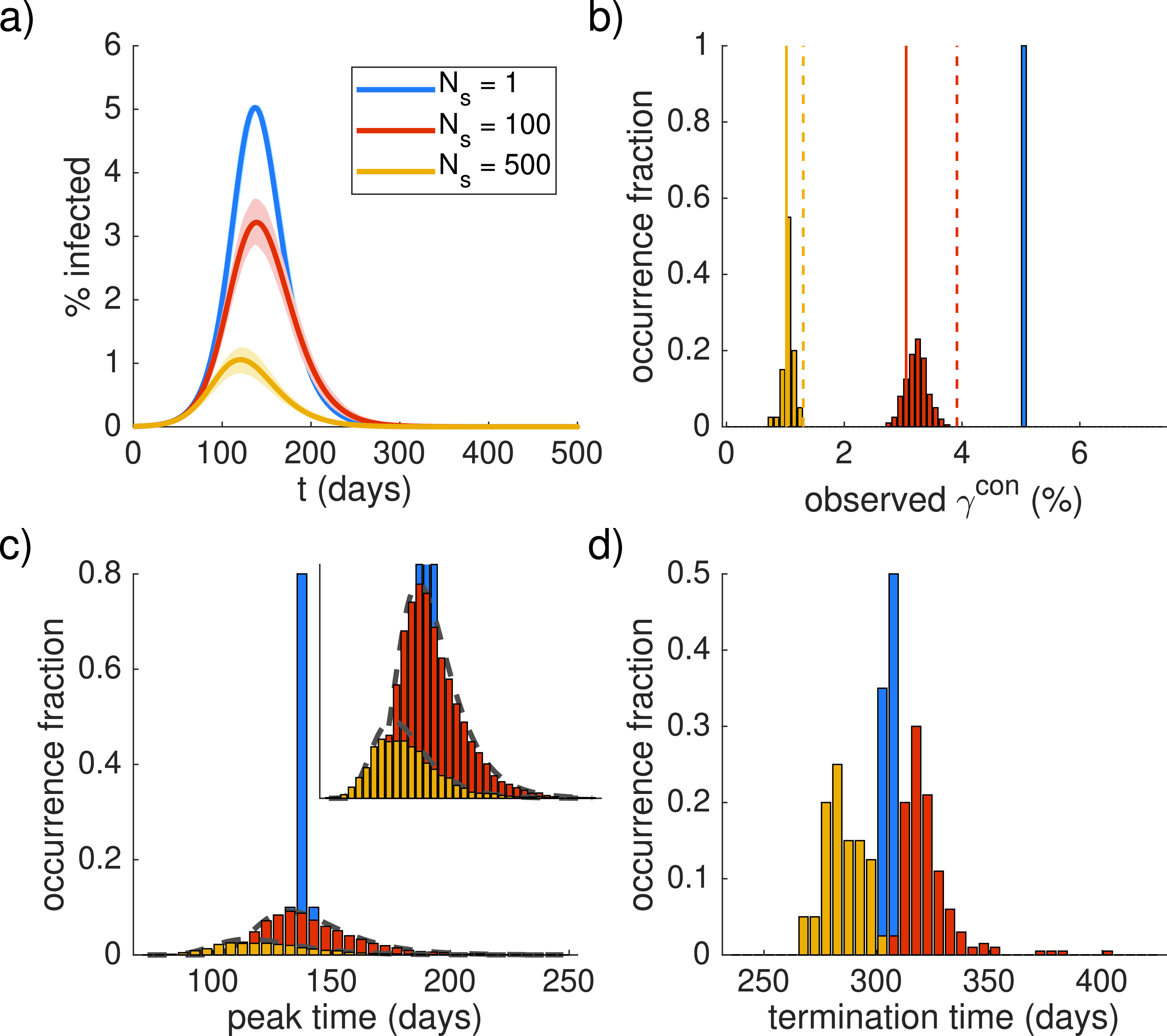
FIG. 2.

Epidemics for different subdivisions of the population. $N=8000000$, $b=0.2$, $k=0.14$, three different values of $N_s=20$, 200, and 40 individual simulations for $N_s=1$, $N_s=100$, and $N_s=500$, respectively. (a) Time courses (solid lines) and 2.5/97.5 percentiles (shading). (b) Distributions of the observed peak percentage ${\gamma }^{\text{con}}$ (in the whole population). The occurrence fraction indicates the fraction of simulations. Analytical estimates for ${\gamma }^{\text{ext}}$ (dashed lines), Eq. (6), and ${\gamma }^{\text{con}}$ (solid lines), Eq. (9), assume $g_n$ according to a binomial distribution. (c) Distribution of peak times in the sub-populations. The inset provides an enlarged y-axis. Dashed lines indicate analytical approximation, Eq. (8), assuming a uniform $n=I_0/N_s$ for each case. (d) Distribution of termination times, defined as the time when $I$ in the total population drops below $I_0$.