Figure 2:

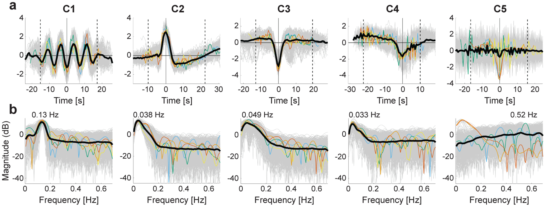
(a) Visualization of the representative temporal patterns (the most important temporal characteristics) of temporal primitives, which are component-specific spatio-temporally-local nonlinear temporal structures learned by the nonlinear feature extractor (CNN). They were represented by taking an average of time fragments whose (unmixed) feature values were very large at each component dimension. Gray thin lines are the individual input time series which produced the top-0.0001% highest component activities in the whole dataset. The colored thin lines indicate the samples with the very highest activations (1st–5th: red, orange, yellow, green, and blue). Considering the well-known property of shift-invariance of CNNs (see Fig. 4a for further evaluation), all samples were temporally shifted so as to maximize their cross correlations to the reference signal, i.e. the one with the highest activity (red sample). The black thick line shows their sample average after the temporal shifting. Two dotted vertical lines indicate the edges of a temporal window whose width is the same as the width of the receptive field of the feature extractor (~ 32 s); the (absolute) peak point inside the window was selected as the reference point (0 s). We can see that the average temporal patterns inside the windows show clear differences across components, and are hereafter used as the representative temporal patterns of the temporal primitives. (b) The representative frequency spectra of the temporal primitives. The spectrum was estimated for each of shift-adjusted inputs corresponding to those in a (see Section 2.9 for the shift-adjustment). As with a, the gray thin lines are the individual plots, the colored thin lines indicate the samples with the very highest activations, and the black thick line shows their average. The peak frequency of the average spectrum was displayed on the line.