FIGURE 1.

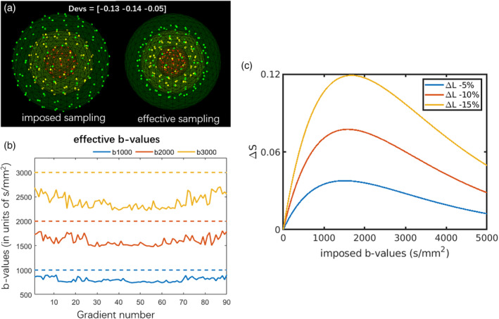
An example of the (a) imposed sampling and the effective sampling with ΔL(r) = diag ([−0.13, −0.14, −0.05]) with three shells. (b) The effective b‐values in each gradient direction (solid line) versus the imposed b‐values (dashed line), due to the gradient deviations, the effective sampling does not adhere to “shells.” (c) Absolute signal changes as a function of the imposed b‐value in the presence of gradient nonlinearities, that is, ΔS = exp(−bL²D) − exp(−bD), where a mono‐exponential signal decay was simulated with D = 0.7 × 10⁻³ mm²/s and L = 1 + ΔL. The signal deviations depend both on the gradient deviations and the b‐values, and the maximum deviation in this scenario occurs at b =  − log(1/L²)/(D * (L² − 1))