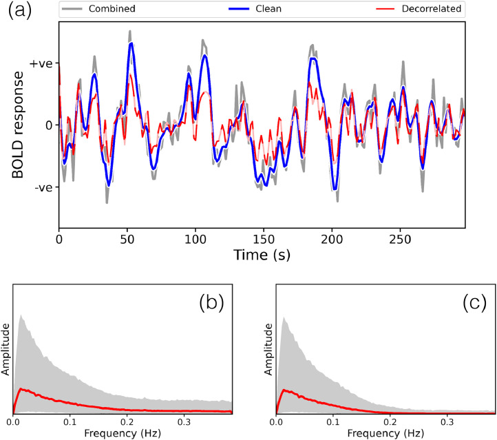
Fig. 15.

Example PFM time courses, and observed frequency content, from the active-state data. Panel (a): Example time course for one mode in one run. ’Combined’ refers to the time course which includes the noise terms (${\mathit{A}}^{\left(sr\right)}={\mathit{B}}^{\left(sr\right)}+{\mathit{\xi }}^{\left(sr\right)}$), ’clean’ refers to the BOLD portion specifically (B^(sr)), while ’decorrelated’ refers to the clean time course after correcting for the temporal autocorrelation induced by the HRF (${\mathit{B}}^{\left(sr\right)}{\mathit{K}}_{\mathit{B}}^{-\frac{1}{2}}$). Panels (b) & (c): Frequency content of the combined and clean time courses respectively, pooled over all runs and subjects. The magnitude of the DFT coefficients are calculated for each time course, and for visualisation purposes, we fit a gamma distribution to the histogram of observed magnitudes for each frequency bin. The mode of this distribution is plotted in red, and the grey region represents the 95% highest density interval (Kruschke, 2014).