General regression model for the subdistribution of a competing risk under left-truncation and right-censoring

Summary

Left-truncation poses extra challenges for the analysis of complex time-to-event data. We propose a general semiparametric regression model for left-truncated and right-censored competing risks data that is based on a novel weighted conditional likelihood function. Targeting the subdistribution hazard, our parameter estimates are directly interpretable with regard to the cumulative incidence function. We compare different weights from recent literature and develop a heuristic interpretation from a cure model perspective that is based on pseudo risk sets. Our approach accommodates external time-dependent covariate effects on the subdistribution hazard. We establish consistency and asymptotic normality of the estimators and propose a sandwich estimator of the variance. In comprehensive simulation studies we demonstrate solid performance of the proposed method. Comparing the sandwich estimator with the inverse Fisher information matrix, we observe a bias for the inverse Fisher information matrix and diminished coverage probabilities in settings with a higher percentage of left-truncation. To illustrate the practical utility of the proposed method, we study its application to a large HIV vaccine efficacy trial dataset.

1. Introduction

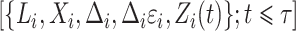
Delayed entries arise in medical studies when individuals come under observation some time after the initial event. The time of the initial event is referred to as the left-truncation time or the delayed entry time, and we denote it by . We consider a competing risks setting, in which individuals are exposed to several distinct event types, denoted by , and only the first-occurring event is observable at time . Individuals are subject to independent right-censoring at . Defining and , we observe only for those individuals with . Such a setting is referred to as a competing risks setting with left-truncated and right-censored data. Individuals with are subject to left-truncation. We will make the common assumption that and are independent given a vector of covariates .

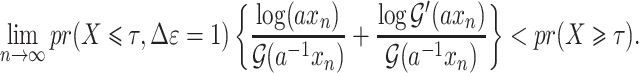
With a sample that represents only those individuals whose event and censoring times exceed the left-truncation time, it is well known that delayed entries need to be taken into account when fitting survival regression models. For the analysis of survival data with independent left-truncation and right-censoring and, without competing risks, a conditional likelihood approach was proposed by Andersen et al. (1988, 2013), Keiding & Gill (1990) and Owen (2001), among others. In particular, one can estimate the regression parameters in proportional hazards models using a conditional partial likelihood, where individuals are included in the risk set from their time of entrance until an event of interest or a censoring is observed.

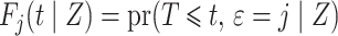
A common approach used in competing risks settings with independent right-censoring is to model the cause-specific hazard , which can be interpreted as the instantaneous risk of dying from cause at time conditional on being alive at . The cumulative incidence function, defined as   is a complex function of all cause-specific hazards. Therefore, estimated parameters targeting the cause-specific hazard cannot be interpreted with regard to the corresponding cumulative incidence function. An alternative approach models the subdistribution hazard for the event of interest,

as defined by Gray (1988), which is the instantaneous risk of experiencing an event of interest at time conditional on not having experienced an event of interest until . The subdistribution hazard is directly related to the corresponding cumulative incidence function through 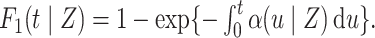Regression parameters targeting the subdistribution hazard are thus directly interpretable with regard to the cumulative incidence function. The subdistribution hazard is also linked to a cure model formulation of the competing risks setting (Bellach et al., 2019) and may be interpreted as the hazard of the event time as in Fine & Gray (1999).

Regression modelling for the subdistribution of a competing risk with independent left-truncation and right-censoring has so far been investigated only for the proportional hazards model (Geskus, 2011; Zhang et al., 2011). As the proportional hazards assumption is not valid in general, it is of interest to consider a more general direct regression model. Moreover, the existing literature does not provide intuition for the proposed weights, and in particular the weighted risk set appears to be unexplained. The purpose of this paper is to give comprehensible arguments for the proposed weights and risk sets, and to derive estimators for a general direct regression model targeting the subdistribution hazard based on a conditional nonparametric maximum likelihood procedure.

We first investigate a competing risks model in which the competing risk event is associated with a cure event. This is frequently the case with infectious diseases. As a historic example, Edward Jenner’s observation that prior infection with cowpox confers protective immunity against smallpox played a pivotal role in the development of the smallpox vaccine, which led to the eradication of smallpox in 1980. A more recent example is vaccination against the dengue virus; epidemiological data support the idea that disease caused by a given dengue genotype prevents disease due to other dengue genotypes within the same serotype (Juraska et al., 2018).

In the cure model setting, left-truncation and right-censoring times can be observed independently of the cure event. Cured individuals with and are incorporated into the risk set, which is denoted by . It is always possible to determine the size of such a risk set from the observed data, although the size of the cure fraction may be unknown. For the competing risks model, individuals with a previous competing risk event are incorporated into the risk set like a cure fraction, as they are no longer exposed to the event of interest. It should be noticed that the terms risk process and risk set are rooted in the tradition of survival analysis and should not be understood in a literal sense. The risk set in a subdistribution hazard model consists of those individuals who have not experienced an event of interest up to time , and may never experience an event of interest because of a cure event or competing risk event prior to . In particular, not all individuals in the risk set are actually at risk for the event of interest.

First, we derive the conditional likelihood function for the cure model, adhering to the principle that the true parameter can be estimated efficiently by the value that maximizes the probability of the observed data. Second, we study the classical competing risks setting, where the occurrence of any event would terminate observation. We use the cure model to obtain new insights into the direct competing risks regression model with left-truncated and right-censored data. For estimation, we weight using the observed data, mimicking the structure that would have occurred in the cure model setting, and define the pseudo risk set. Specifically, the expected number of individuals in the pseudo risk set is by construction equal to the expected number of individuals in the corresponding cure model risk set.

We derived the proposed weighted conditional nonparametric maximum likelihood estimators using the R (R Development Core Team, 2020) function optim with the method specified as BFGS, which utilizes the Broyden–Fletcher–Goldfarb–Shanno algorithm, a quasi-Newton method. For all simulation studies and clinical trial data that we investigated, the optimization worked very reliably.

2. Pseudo risk set and weighted likelihood function

2.1. Cure model with complete data

We start by investigating a competing risks model in which the competing risk event is connected to the cure of the subject. Denoting an event of interest by and the competing event by , the cure event at implies that , although the subject is still observable. Let denote the duration of the study, with administrative censoring at . For settings with only administrative censoring at , we have and . For a random sample , the observed data are for and for . The process counting the events of interest is where . The individual at-risk process is  , and is the cardinality of the risk set for .

We denote the cumulative subdistribution hazard for the event of interest by and define . As argued in Bellach et al. (2019), is the compensator of with respect to the filtration , and the Nelson–Aalen estimator for the cumulative subdistribution hazard can be derived from the Doob decomposition , with denoting the martingale. A likelihood function as in Bellach et al. (2019, § 2.1) can be derived by considering that the contribution for an event of interest is with , and the contribution for a cure event or administrative censoring at is . The estimator for the cumulative subdistribution hazard that is obtained from maximizing this likelihood function is equivalent to the Nelson–Aalen estimator.

2.2. Cure model with independent left-truncation and right-censoring

With independent left-truncation and right-censoring, we have and . The observed data are for subjects , for subjects and 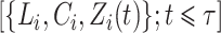for subjects . The process counting the observed events of interest is denoted by with , and 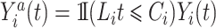is the individual at-risk process for subject . Then is the cardinality of the risk set

(1)

(2)

The risk set in (1) is based on observable data. Subjects enter the study at independently of a possible cure event and remain in the risk set until an event of interest is observed at or until censoring at . The size of the cure fraction may be unobservable for the theoretical decomposition (2), with subjects entering the study after the cure event. For modelling of the subdistribution hazard, however, only knowledge about the size of the risk sets is required, which can be obtained from (1) regardless of the specific decomposition (2).

A Nelson–Aalen estimator for the cumulative subdistribution hazard can be derived from the weighted Doob decomposition . The same estimate may also be derived from a weighted conditional likelihood function obtained by considering that the contribution for an observed event of interest at is with , the contribution for an observed censoring is , and the contribution for a cured individual with is , regardless of whether the cure event occurred before or after the entrance time . We thus obtain the conditional likelihood function

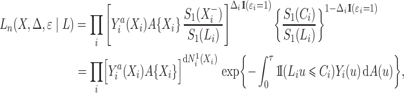where the cumulative baseline subdistribution hazard is approximated by a step function with jumps at the observed event times, which are denoted by .

2.3. Left-truncated and right-censored competing risks data

Modelling the subdistribution hazard for the competing risks model requires a reconstruction of the cure model risk set, where the cure fraction consists of . For the competing risks model, however, only subjects with are observable, and in particular subjects are assigned to the cure fraction. The observed data are for subjects and for subjects .

To maintain the cure model structure, an adjustment for hypothetical left-truncation after competing risk events and right-censoring of individuals in the cure fraction is required. We apply inverse probability of censoring weighting. A weight function that consistently estimates , where , would be justified by . We make the decomposition , with simplified weights , to define the pseudo risk set

The process counting the observable events of interest is defined by , with . A Nelson–Aalen-type estimator for the cumulative subdistribution hazard is obtained from the weighted Doob decomposition , and may also be derived from the weighted conditional likelihood function from § 2.2, where the risk set indicator is replaced by :

A product limit estimator for the cumulative incidence function can be derived based on the Nelson–Aalen-type estimator for the subdistribution hazard. Zhang et al. (2009) and Geskus (2011) proved its equivalence to the fully efficient Aalen–Johansen estimator. This suggests that the weighted conditional likelihood function is a promising candidate for likelihood-based inference on the subdistribution hazard.

3. Definition and estimation of the weights

We use the following representation of the theoretical weights:

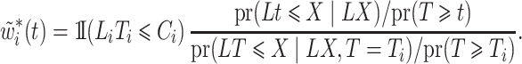Denoting the number of observable events by 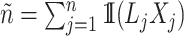and the number of observable individuals by 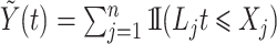, we estimate consistently by . The unconditional probabilities and can be estimated with the product limit estimator. Let be the process counting the competing risk events. We obtain the estimated weights

where is the left-truncated version of the product limit estimator for the overall survival, as proposed by Zhang et al. (2011). Decomposing the weight yields , with

Geskus (2011) introduced weights based on the product limit estimator estimating and the inverse product limit estimator of the delayed entries estimating , which had previously been investigated by Keiding & Gill (1990) for a model with independent left-truncation and no censoring. A common assumption for left-truncated and right-censored data is independence of and , but not independence of and . For this reason, the validity of the weights

which may be decomposed as with

is not immediately apparent. A theoretical justification using results of He & Yang (1998) would require independence of and . Interestingly, the weights and are equivalent with continuous , as we prove in the Supplementary Material, thereby justifying the weights proposed by Geskus (2011).

For a competing risks model with only left-truncation and no right-censoring, the weights simplify; for example, the theoretical weights in this case are .

4. General regression model

We consider estimation of a general model for the cumulative subdistribution hazard

as in Bellach et al. (2019), akin to a general semiparametric regression model for survival and recurrent event data without left-truncation and competing risks, which has been investigated by Zeng&Lin (2006); here is a vector of unknown regression parameters, is an unspecified increasing function, and is a thrice continuously differentiable and strictly increasing function with , and . Regularity conditions for this model, which are considerably weaker than those in Zeng & Lin (2006), are specified in the Appendix. Special cases of the general model include the Box–Cox transformation models with link function 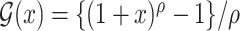for , and the logarithmic transformation models with link function 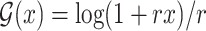for  (Chen et al., 2002). The Fine–Gray model under left-truncation and right-censoring (Geskus, 2011; Zhang et al., 2011) is also a special case. In particular, the proportional hazards model is the Box–Cox transformation model with and the limiting logarithmic transformation model with , while the proportional odds model is the logarithmic transformation model with and the limiting Box–Cox transformation model with . If is differentiable, the instantaneous subdistribution hazard rate is defined by

(3)

where 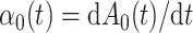denotes the baseline subdistribution hazard and is a vector of external time-dependent or time-independent covariates.

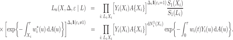
For the cure model with independent left-truncation and right-censoring, we define to obtain the conditional loglikelihood

By rearranging terms in the second sum, this can be written as

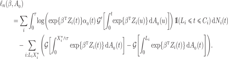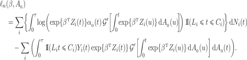
With independently left-truncated and right-censored competing risks data, we obtain

(4)

For statistical inference, the baseline subdistribution hazard is approximated by a sequence of step functions, and the weighted nonparametric maximum likelihood estimator is obtained by maximizing the discretized loglikelihood function with respect to and the jump sizes . In the Appendix and Supplementary Material we prove the following theorem.

Theorem 1.

The weighted nonparametric maximum likelihood estimator   is uniformly consistent.

With an application of Lemma S2 from the Supplementary Material, which is based on Theorem 3.3.1 in van der Vaart & Wellner (1996), we derive the following theorem.

Theorem 2.

We have that   converges weakly to a zero-mean Gaussian process.

We prove these theorems first for the cure model set-up, thereby adapting arguments by Murphy (1994, 1995), Parner (1998), Zeng & Lin (2006) and Bellach et al. (2019). These results are then adapted to the direct competing risks regression model, which has a similar mathematical structure.

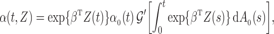
To obtain weak convergence and for variance estimation, we consider the linear functionals

where , with being a function in the Skorohod space and . Let be the ordered times for the event of interest and let be the number of such events. Defining a vector with  , the asymptotic variance of the linear functional can be estimated by the sandwich estimator

where is the observed Fisher information matrix with respect to and the jump sizes, and is the estimated variance of the score with respect to and the jump sizes, with , and denoting the components of the independent and identically distributed decomposition given in the Supplementary Material. Analogously, we obtain the estimator for the covariances of and , with and with corresponding vectors :

For the cure model, the sandwich estimator simplifies to the inverse Fisher information. However, for the competing risks model with independent left-truncation and right-censoring, the middle term contains additional terms reflecting the extra variability from the estimated weights.

5. Simulation studies

We conducted simulation studies for the Fine–Gray model and for the proportional odds model to evaluate the bias, the empirical and model-based variances, and the coverage probabilities of the proposed method for different sample sizes. We considered settings with two different event types. All simulation results are based on 1000 repetitions.

For our first set of simulations with fixed covariates, displayed in Table 1, we used the model formulations in Fine & Gray (1999) and Fine (2001), which are specified in the Supplementary Material. The covariates and   were generated independently from a standard normal distribution. For the second set of simulations, displayed in Table 2, we developed a new method to generate event times for competing risks models with binary time-dependent covariates, the details of which are given in the Supplementary Material. We generated from a standard normal distribution and generated as a time-dependent covariate with one transition from 0 to 1, thereby assuming that the covariate process is observable after the competing risk event. The transition time for was generated from a standard exponential distribution.

Table 1.

Simulation results for the Fine–Gray and proportional odds models. For columns 3–8, , , is generated from with probability and set to zero otherwise, and with ; approximately are left-truncated, are censored, are events of interest and are competing events. For columns 9–14, , , is generated from with probability and set to otherwise, and with ; approximately are left-truncated, are censored, are events of interest and are competing events

		Fine–Gray model						Proportional odds model
Size	Parameter	Bias	SE			CP	CP	Bias	SE			CP	CP

Bias, absolute value of bias; SE, empirical standard error; , inverse Fisher information; , sandwich estimator; CP and CP, coverage probabilities of confidence intervals for and , respectively; all results are multiplied by .

Table 2.

Results of simulation studies with external time-dependent covariates. For columns 3–8, , , is generated from with probability and set to otherwise, and with ; approximately are left-truncated, are censored, are events of interest and are competing events. For columns 9–14, , , is generated from with probability and set to otherwise, and with ; approximately are left-truncated, are censored, are events of interest and are competing events

			Fine–Gray model						Proportional odds model
Size	Parameter	Bias	SE			CP	CP	Bias	SE			CP	CP

Bias, absolute value of bias; SE, empirical standard error; , inverse Fisher information; , sandwich estimator; CP and CP, coverage probabilities of confidence intervals for and , respectively; all results are multiplied by .

In all simulation studies the performance of the weighted nonparametric maximum likelihood estimator is solid, even for small sample sizes, in terms of the bias, and the standard errors and coverage probabilities of the proposed sandwich estimator. The bias is generally small, the standard errors decrease at rate , the proposed sandwich estimators are close to the empirical variance estimators, and the coverage probabilities are close to the nominal level of , particularly for sample sizes , and .

Comparing the results for the estimated variances, in particular for the additional simulation studies presented in the Supplementary Material, it is observed that the proposed sandwich estimator has the desired properties, while the inverse Fisher information matrix underestimates the variance of the parameter estimates, and, moreover, the coverage probabilities are clearly smaller than the desired value of .

Simulation results reported in the Supplementary Material confirm our theoretical results on the equivalence of the weights proposed by Geskus (2011) and Zhang et al. (2011).

6. Application to HIV vaccine efficacy trial data

We analysed data from the HVTN 503 preventive HIV vaccine efficacy trial in South Africa, to assess how participant factors are associated with the time from reaching adulthood to diagnosis of genotype-specific HIV-1 infection. These data, from 784 individuals screened at age 18 and above, are left-truncated because only those who test negative for HIV-1 are eligible to enrol in the trial. It was of particular interest to investigate the efficacy of the vaccine and the effects of sex at birth, and body mass index at enrolment on the time to infection with the HIV-1 169K virus, which has a vaccine-matched residue at position 169 of the V2 loop, compared with the effects on the time to infection with the HIV-1 K169! virus, which has a vaccine-mismatched residue at position 169. This question is relevant because an HIV vaccine is currently undergoing testing for efficacy in the HVTN 702 randomized, placebo-controlled trial in South Africa, and it is hypothesized that the efficacy of this vaccine against the virus type HIV-1 169K is superior to that against type HIV-1 K169!, because a previous trial of a similar HIV vaccine showed greater efficacy against HIV-1 type 169K (Rolland et al., 2012).

A total of 28 infections with HIV-1 virus type 169K and 15 infections with HIV-1 virus type K169! were observed. We conducted backward selection starting with the covariates assignment to vaccine, sex at birth and body mass index, and then removed the last, which was clearly nonsignificant.

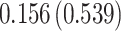
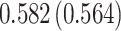
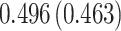
Our findings, displayed in Tables 3 and 4, indicate that women in South Africa tend to be infected at earlier ages than men. For HIV-1 type 169K, the results can be interpreted as an increase in the expected subdistribution hazard for women, with , and an increase in the expected odds ratio, with . For HIV-1 type K169! this would be interpreted as a increase in the expected subdistribution hazard for women, with , and a increase in the expected odds ratio, with . 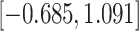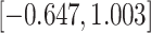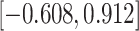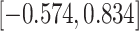As illustrated in Fig. 1, for infection with HIV-1 type 169K, the fit of the model may be improved with a logarithmic transformation and parameter , while for infection with HIV-1 type K169! a Box–Cox transformation with a larger parameter may yield a moderately improved fit over the Fine–Gray and proportional odds models. The observed direct association with risk of being female in comparison to being male was therefore significantly greater for HIV-1 type 169K than for HIV-1 type K169!. The result that women and men have different risks especially for HIV-1 type 169K motivates further exploratory analyses in the HVTN 702 trial, including assessment of whether sex modifies vaccine efficacy against HIV-1 type 169K.

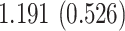
Table 3.

Time to infection with vaccine-matched virus (, 169K HIV-1 infection): effect of vaccination and of sex at birth on time to HIV-1 infection; reported are parameter estimates (with standard errors in parentheses) for different semiparametric transformation models and the estimated confidence intervals

		Logarithmic transformation		Box–Cox transformation
				PO model	FG model
Loglik
Treat
	CI
Sex
	CI

PO, proportional odds; FG, Fine–Gray; Loglik, loglikelihood; Treat, vaccination treatment; Sex, sex at birth (indicator of female); CI, confidence interval.

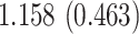
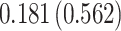
Table 4.

Time to infection with vaccine unmatched virus (, K169! HIV infection): effect of vaccination and of sex at birth on time to HIV-1 infection; reported are parameter estimates (with standard errors in parentheses) for different semiparametric transformation models and the estimated confidence intervals

		Logarithmic transformation		Box–Cox transformation
			PO model	FG model
Loglik
Treat
	CI
Sex
	CI

PO, proportional odds; FG, Fine–Gray; Loglik, loglikelihood; Treat, vaccination treatment; Sex, sex at birth (indicator of female); CI, confidence interval.

Fig. 1.

Model selection with Akaike criterion for the HIV vaccine data: the upper panels are for HIV-1 type 169K and the lower panels for HIV-1 type K169!; the left panels show logarithmic transformation models and the right panels Box–Cox transformation models.

7. Discussion

Any cure model may be interpreted as a competing risks model where the competing risk event is the cure. Therefore, the subdistribution hazard approach proposed in § 2.2 can be applied to any cure model under left-truncation and right-censoring.

A direct relation between the subdistribution hazard and the cumulative incidence function can be established for either time-independent covariates, such as baseline covariates, or external time-dependent covariates. But this is not possible for internal time-dependent covariates, as discussed in Bellach et al. (2019). It is well known that even in survival settings without competing risks, regression parameters for the hazard rate in the presence of internal time-dependent covariates are not interpretable with regard to the underlying distribution; see, for instance, Kalbfleisch & Prentice (2002).

The general regression model can be extended to a model for the marginal mean intensity for recurrent event data with competing terminal events under left-truncation and right-censoring. For the marginal mean intensity, defined as where denotes the process counting the number of recurrent events, the usual relationship with the marginal mean is retained; i.e., 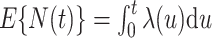. A slightly modified version of the weighted loglikelihood function (4) may be applied to estimate the regression parameters for the general model for the marginal mean intensity as defined in (3).

Appendix

Model conditions

 

Condition A1.

The cumulative baseline is a strictly increasing and continuously differentiable function, and lies in the interior of a compact set .

Condition A2.

The vector of covariates is with probabilty one of bounded variation on the observed interval . In combination with Condition A1 this implies that there is a constant such that .

Condition A3.

The endpoint of the study is chosen in such a way that with probability one there exists a constant such that and . There is a finite partition of the interval with for some .

Condition A4.

The function is thrice continuously differentiable and strictly increasing, with , and . Moreover, one of the following conditions holds:

• (i) for ;

• (ii) for and, in addition, for any and any sequence with as ,

  (A1)

Condition A5.

(Identifiability). If a vector and a deterministic function , , exist such that with probability one, then and for -almost all , where denotes Lebesgue measure. This condition rules out perfect multicollinearity of the covariates for -almost all .

Condition A6.

Let denote a vector in and let . For a subset of nonzero Lebesgue measure, for all we have that

Existence of the weighted nonparametric maximum likelihood estimator and consistency

We first ascertain that is bounded almost surely on . As a consequence, all estimated jump sizes must be finite. By the Helly–Bray lemma we obtain that for every sequence there exist a subsequence and such that . Together with Condition A1 this implies sequential compactness for , which means that for every sequence there exist a subsequence and such that . Using a Kullback–Leibler argument, one can then conclude that every subsequence converges to the true parameter . As is a continuous and increasing function, we obtain uniform almost sure convergence for the cumulative baseline hazard and almost sure convergence for .

Let be a constant such that . We define 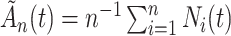and consider the sequence . Under Condition A4(i) the sequence is bounded above by

and under Condition A4(ii) the sequence is bounded above by

In both cases the upper bound would become infinitely small if , which means that would go to as . This contradicts the definition of as a maximum likelihood estimator. Therefore is bounded almost surely on .

Writing and , we define the Kullback–Leibler distance for the cure model with independent left-truncation and right-censoring as

where is the subdistribution density for the event of interest. In the Supplementary Material we prove that and , and establish the identifiability, namely that if then . For the competing risks model with independent left-truncation and right-censoring, we define

Consistency then follows from the asymptotic equivalence of and .

Weak convergence to a Gaussian process

Let denote the space of elements with and . A norm on is then defined by , where denotes the Euclidean norm and the total variation norm. For we define . The parameter space is . For we define , so that . One-dimensional submodels of the form are considered with to define the empirical score operator

for a measurable function , where is the component related to the derivative with respect to and is the component related to the derivative along the submodel for , as stated in the Supplementary Material. The limiting version is defined by replacing the empirical measure by the probability measure . It is then sufficient to verify the conditions of Lemma S2 in the Supplementary Material for weighted -estimators.

To verify condition in Lemma S2, note that as our model is based on independent and identically distributed observations, it is sufficient to verify the two conditions of Lemma S3. Arguments like those in van der Vaart & Wellner (1996) and Kosorok (2008) along the lines of Donsker preservation theorems are immediately applicable. The second condition of Lemma S3 immediately follows, as pointwise convergence can be strengthened to convergence by dominated convergence. By the Donsker theorem, converges in distribution to the tight random element . Also by the Donsker theorem, converges in distribution to a tight random element . Joint convergence follows from the asymptotic linearity of the two components marginally, together with the fact that the composition of two Donsker classes is also Donsker. By definition . As argued in Parner (1998), from the Kullback–Leibler information being positive and by interchanging expectation and differentiation, we obtain .

To show continuous invertibility of and , it suffices to prove the invertibility of the operator corresponding to the cure model, as the scores for the cure model and for the competing risks model with left-truncation and right-censoring are asymptotically equivalent. Therefore, and are also asymptotically equivalent. The continuous Gateaux derivatives are provided in the Supplementary Material. Gateaux differentiability can be strengthened to Frechét differentiability with an additional continuity condition.

Thus, from Lemma S2 we obtain weak convergence of , and the covariances for the limiting process with and are

for  (Kosorok, 2008).

Supplementary material

Supplementary material available at Biometrika online includes proofs of Theorems 1 and 2, details on the sandwich estimator for the variance, results of additional simulation studies, and a proof of the equivalence of the weights proposed by Geskus (2011) and Zhang et al. (2011).

References

- Andersen, P. K., Borgan, Ø., Gill, R. D. & Keiding, N. (1988). Censoring, truncation and filtering in statistical models based on counting processes. Contemp. Math. 80, 19–60. [Google Scholar]
- Andersen, P. K., Borgan, Ø., Gill, R. D. & Keiding, N. (2013). Statistical Models Based on Counting Processes. New York: Springer. [Google Scholar]
- Bellach, A., Kosorok, M. R., Rüschendorf, L. & Fine, J. P. (2019). Weighted NPMLE for the subdistribution of a competing risk. J. Am. Statist. Assoc. 114, 259–70. [DOI] [PMC free article] [PubMed] [Google Scholar]
- CASCADE Collaboration (2006). Effective therapy has altered the spectrum of cause-specific mortality following HIV seroconversion. AIDS 20, 741–9. [DOI] [PubMed] [Google Scholar]
- Chen, K., Jin, Z. & Ying, Z. (2002). Semiparametric analysis of transformation models with censored data. Biometrika 89, 659–68. [Google Scholar]
- Fine, J. P. (2001). Regression modeling of competing crude failure probabilities. Biostatistics 2, 85–97. [DOI] [PubMed] [Google Scholar]
- Fine, J. P. & Gray, R. J. (1999). A proportional hazards model for the subdistribution of a competing risk. J. Am. Statist. Assoc. 94, 496–509. [Google Scholar]
- Geskus, R. B. (2011). Cause-specific cumulative incidence estimation and the Fine and Gray model under both left truncation and right censoring. Biometrics 67, 39–49. [DOI] [PubMed] [Google Scholar]
-
Gray, R. J. (1988). A class of
-sample tests for comparing the cumulative incidence of a competing risk. Ann. Statist. 16, 1141–54. [Google Scholar]
- He, S. & Yang, G. L. (1998). Estimation of the truncation probability in the random truncation model. Ann. Statist. 26, 1011–27. [Google Scholar]
- Juraska, M., Magaret, C. A., Shao, J., Carpp, L. N., Fiore-Gartland, A., Benkeser, D., Girerd-Chambaz, Y., Langevin, E., Frago, C., Guy, B. et al. (2018). Viral genetic diversity and protective efficacy of a tetravalent dengue vaccine in two phase 3 trials. Proc. Nat. Acad. Sci. 115, E8378–87. [DOI] [PMC free article] [PubMed] [Google Scholar]
- Kalbfleisch, J. D. & Prentice, R. L. (2002). The Statistical Analysis of Failure Time Data. Hoboken, New Jersey: John Wiley & Sons, 2nd ed. [Google Scholar]
- Keiding, N. & Gill, R. D. (1990). Random truncation models and Markov processes. Ann. Statist. 18, 582–602. [Google Scholar]
- Kosorok, M. R. (2008). Introduction to Empirical Processes and Semiparametric Inference. New York: Springer. [Google Scholar]
- Murphy S. A. (1994). Consistency in a proportional hazards model incorporating a random effect. Ann. Statist. 22, 712–31. [Google Scholar]
- Murphy S. A. (1995). Asymptotic theory of the frailty model. Ann. Statist. 23, 182–98. [Google Scholar]
- Owen, A. B. (2001). Empirical Likelihood. Boca Raton, Florida: Chapman & Hall/CRC. [Google Scholar]
- Parner, E. (1998). Asymptotic theory for the correlated gamma-frailty model. Ann. Statist. 26, 183–214. [Google Scholar]
- R Development Core Team (2020). R: A Language and Environment for Statistical Computing. R Foundation for Statistical Computing, Vienna, Austria. ISBN 3-900051-07-0. http://www.R-project.org. [Google Scholar]
- Rolland, M., Edlefsen, P. T., Larsen, B., Tovanabutra, S., Sanders-Buell, E., Hertz, T., Decamp, A. C., Carrico, C., Menis, S., Magaret, C. A. et al. (2012). Increased HIV-1 vaccine efficacy against viruses with genetic signatures in Env V2. Nature 490, 417–20. [DOI] [PMC free article] [PubMed] [Google Scholar]
- van der Vaart, A. W. & Wellner, J. A. (1996). Weak Convergence and Empirical Processes. New York: Springer. [Google Scholar]
- Zeng, D. & Lin, D. Y. (2006). Efficient estimation of semiparametric transformation models for counting processes. Biometrika 93, 627–40. [Google Scholar]
- Zhang, X., Zhang, M. J. & Fine, J. P. (2009). A mass redistribution algorithm for right-censored and left-truncated time to event data. J. Statist. Plan. Infer. 139, 3329–39. [DOI] [PMC free article] [PubMed] [Google Scholar]
- Zhang, X., Zhang, M. J. & Fine, J. P. (2011). A proportional hazards regression model for the subdistribution with right-censored and left-truncated competing risks data. Statist. Med. 30, 1933–51. [DOI] [PMC free article] [PubMed] [Google Scholar]
Associated Data
This section collects any data citations, data availability statements, or supplementary materials included in this article.