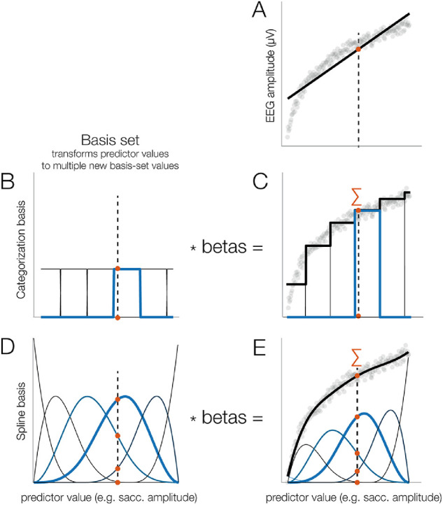
Figure 5.

Using splines to model nonlinear effects, illustrated here for simulated data. (A) Example of a relationship between a predictor (e.g., saccade amplitude) and a dependent variable (e.g., fixation-related P1). As can be seen, a linear function (black line) fits the data poorly. The dashed vertical line indicates some example value of the independent variable (IV) (e.g., a saccade amplitude of 3.1°). (B) Categorization basis set. Here, the range of the IV is split up into non-overlapping subranges, each coded by a different predictor that is coded as 1 if the IV value is inside the range and as 0 otherwise. The IV is evaluated at all functions, meaning that, in this case, the respective row of the design matrix would be coded as [0 0 0 1 0 0]. (C) After computing the betas and weighting the basis set by the estimated beta values, we obtained a staircase-like fit, clearly better than the linear predictor, but still poor. (D) Spline basis set. The range of the IV is covered by several spline functions that overlap with each other. Note that the example value of the IV (3.1°) produces non-zero values at several of the spline predictors (e.g., [0 0 0.5 0.8 0.15 0]). (E) After computing the betas and weighting the spline set by the betas, we obtain a smooth fit.