Urban-scale variation in pollen concentrations: A single station is insufficient to characterize daily exposure

Abstract

Epidemiological analyses of airborne allergenic pollen often use concentration measurements from a single station to represent exposure across a city, but this approach does not account for the spatial variation of concentrations within the city. Because there are few descriptions of urban-scale variation, the resulting exposure measurement error is unknown but potentially important for epidemiological studies. This study examines urban scale variation in pollen concentrations by measuring pollen concentrations of 13 taxa over 24-hr periods twice weekly at 25 sites in two seasons in Detroit, Michigan. Spatio-temporal variation is described using cumulative distribution functions and regression models. Daily pollen concentrations across the 25 stations varied considerably, and the average quartile coefficient of dispersion was 0.63. Measurements at a single site explained 3–85% of the variation at other sites, depending on the taxon, and 95% prediction intervals of pollen concentrations generally spanned one to two orders of magnitude. These results demonstrate considerable heterogeneity of pollen levels at the urban scale, and suggest that the use of a single monitoring site will not reflect pollen exposure over an urban area and can lead to sizable measurement error in epidemiological studies, particularly when a daily time-step is used. These errors might be reduced by using predictive daily pollen levels in models that combine vegetation maps, pollen production estimates, phenology models and dispersion processes, or by using coarser time-steps in the epidemiological analysis.

1. Introduction

Exposure to allergenic pollen can trigger allergic rhinitis, allergic conjunctivitis, and asthma attacks (Bousquet et al. 2008; La Rosa et al. 2013; Linneberg et al. 2002; Salo et al. 2011). Sensitization to pollen is common, and estimates of allergic rhinitis prevalence range from 10 – 30% (D’Amato et al. 2007; Mims 2014). Suffering individuals endure substantial reductions in quality of life and economic productivity (Blaiss et al. 2018; Meltzer 2016; Meltzer et al. 2009), and estimates of the health burden range to 5 million lost school and work days annually in the United States (Nathan 2007). In Sweden, the economic cost of allergic rhinitis alone has been estimated at €1.3 billion annually (Cardell et al. 2016). Epidemiological analyses have linked ambient pollen concentrations to emergency department visits (Darrow et al. 2012; Sun et al. 2016), medication purchases (Ito et al. 2015), allergy symptoms (Werchan et al. 2018), and suicides (Qin et al. 2013).

Most epidemiological studies of allergenic pollen have implicitly assumed that pollen concentrations are uniform across the study area, typically a metropolitan area (Darrow et al. 2012; Guilbert et al. 2016; Osborne et al. 2017; Sakata et al. 2017; Sun et al. 2016) or a larger region (Gleason et al. 2014; Ito et al. 2015). These studies usually compare a time series of pollen concentrations monitored at a single location with health outcomes aggregated across the study area, typically using a daily time-step. Although rarely considered (but see Werchan et al., 2018), intra-urban differences in pollen concentrations can result in substantial exposure measurement error, defined here as the difference between observed and estimated pollen levels at a location. For air pollutants, spatial variability and temporal misalignments associated with the use of a single monitoring station have been long recognized as issues that can bias results (Wilson et al. 2005). Exposure measurement error for airborne pollen can arise for a number of reasons, and information on spatial and temporal variability in pollen concentrations is needed to assess the potential for such effects.

Spatial variation of pollen concentrations has been documented in several studies (Table 1). Three studies collected brief (15 min to 3 hr) measurements sequentially at 6 to 16 sites within a city (Charalampopoulos et al. 2018; Hjort et al. 2015; Katz et al. 2019). Such data can help describe average differences between sites, but not how pollen concentrations vary within a city on a particular day since the measurements are brief and taken at different times. Several other studies used long sampling integration periods (e.g., 5 days – 8 months with gravitational samplers) (Emberlin and Norris-Hill 1991; Katz and Carey 2014; Weinberger et al. 2018; Werchan et al. 2017), which does not show short term variability, e.g., on the daily basis that is commonly used in health studies. Ishibashi et al. (2008) sampled at 78 sites in a city for a 24-hr period, however, sampling was conducted on only two days, and the gravitational samplers used do not measure airborne concentrations and are considered an inaccurate sampling method (Levetin 2004). Several other studies have assessed correlations in airborne pollen concentrations at a handful of sites (Fernández-Rodríguez et al. 2014a; Weinberger et al. 2015), but it is difficult to draw large conclusions about intra-municipal spatial heterogeneity from a small number of sampling sites. Thus, spatial variation on the daily time-step important for health studies remains largely unknown.

Table 1:

Studies that have quantified spatial variation in airborne pollen concentrations on the municipal scale at more than five sites.

Study	Plant type	Number of locations	Sampling approach	Sample integration period	Sampler used
Emberlin and Norris-Hill 1991	Trees, grass	14	simultaneous	7 days	Hyde (gravitational)
Bricchi et al. 2000	Tree	12	simultaneous	7 days	Durham (gravitational)
Ishibashi et al. 2008	Tree	78	simultaneous	1 day*	Durham (gravitational)
Katz and Carey 2014	Ragweed	34	simultaneous	5 days	Durham (gravitational)
Hjort et al. 2015	Grass	16	sequential	30 minutes	Rotorod (rotating impactor)
Werchan et al. 2017	Trees, grass, herbaceous	14	simultaneous	7 days	Durham (gravitational)
Weinberger et al. 2018	Trees	45	simultaneous	8 months	Tauber (gravitational)
Charalampopoulos et al. 2018	Trees	6	sequential	15 minutes	Portable Hirst (suction impactor)
Katz et al. 2019	Trees	13	sequential	3 hours	Rotorod (rotating impactor)

^*Ishibashi et al. (2008) deployed 78 samplers for a 24-hr period, but this was only done once in 2005 and once in 2006.

The temporal variability of pollen levels measured at a single site (and a few sites in several cases) has been well documented, but studies examining how spatial patterns at the urban scale vary over time (i.e., spatio-temporal variation) have mostly been conducted at weekly time steps (Emberlin and Norris-Hill 1991; Werchan et al. 2017). We recently examined effects of intra-urban temperature gradients on the timing of peak pollen release within Detroit, Michigan, which led to differences in pollen concentrations between sites (Katz et al. 2019). However, that study was not designed to describe how spatial patterns of pollen concentrations changed between days. More empirical data are required to describe spatio-temporal variation, such as simultaneous measurements of pollen concentrations at numerous locations over repeated 24-hr periods. If the variation is high, then measurements from a single monitoring location may be a poor proxy for concentrations at other sites.

This study evaluates spatial and spatio-temporal variability of allergenic pollen concentrations by simultaneously measuring airborne pollen concentrations at 25 locations across Detroit, Michigan, USA on 21 sampling days. These data are used to investigate how pollen concentrations differ throughout the city on a daily basis, whether the same sites have consistently higher concentrations, and how well measurements at one site represent levels elsewhere. This information provides insight into the extent of exposure measurement error that can affect epidemiological studies and into the design of and interpretation of data from pollen monitoring networks.

2. Materials and methods

2.1. Study area

The study was conducted in Detroit, Michigan, USA. Tree canopy covers 21.6% of Detroit and vacant lots occupy 16% of land area (Katz and Batterman 2019). Focal taxa (Table 2) include several trees (Acer, Betula, Cupressaceae, Gleditsia, Juglans, Morus, Pinaceae [including Pinus and the morphologically similar genera Abies and Picea but not the morphologically distinct Tsuga], Platanus, Populus, Quercus, Salix, and Ulmus), grasses (Poaceae), and ragweed (Ambrosia); other taxa had low pollen concentrations and are not included. Several taxa (e.g., Acer, Ulmus, and Gleditsia tricanthos) are common street trees in Detroit, whereas others are rare (e.g., Juglans). Plant cover has increased in Detroit neighborhoods as building vacancy has increased over the last three decades (Endsley et al. 2018), and preliminary data from the Urban Forest Inventory and Analysis (Richard McCullough, personal communication) suggest that early successional genera such as Ulmus, Populus, and Morus are especially common among non-street trees in Detroit. The annual average temperature in Detroit is 10.6° C and the average precipitation is 940 mm/yr. Weather during the sampling period is provided in SI 1.

Table 2:

Focal taxa including trees, ragweed, and Poaceae. Tree abundance in Detroit is based on street tree data and does not include trees on private property or in parks.

Focal taxa	Common name	Major pollen producing species	Relative basal area street trees (%)
Acer	Maple	A. saccharinum, A. rubrum, A. saccharum, A. negundo	46.9
Betula	Birch	B. papyrifera, B. nigra	0.1
Cupressaceae	Juniper, arborvitae	Juniperus virginiana, Thuja occidentalis	> 0.1
Gleditsia	Honey locust	Gleditsia tricanthos	10.2
Juglans	Walnut	J. nigra	0.1
Morus	Mulberry	M. alba, M. rubra	0.4
Pinaceae	Pine	Pinus nigra, P. sylvestris, P. strobus, Picea abies	0.2
Platanus	Sycamore, London planetree	P. occidentalis, P. x acerfolia	9.1
Populus	Poplar	P. deltoides, P. alba	2.0
Quercus	Oak	Q. palustris, Q. rubra, Q. macrocarpa, Q. alba, Q. robur	5.6
Salix	Willow	S. matsudana, S. babylonica	0.2
Ulmus	Elm	U. pumila, U. americana, U. rubra	10.4
Ambrosia	Ragweed	A. artemisiifolia, A. trifida	-
Poaceae	Grasses	Dactylis glomerata, Elymus repens, Panicum dichtomiflorum, Poa annua, etc., *	-

^*Personal observation; graminoids were not quantitatively surveyed.

2.2. Pollen collection, samplers, and processing

Pollen was measured at 1.5 m height at 25 sites on volunteers’ property in or immediately adjacent to Detroit (Fig. 1A). While the locations of our sampling sites were constrained to volunteers’ locations (and thus were not randomly selected), they are distributed across a large portion of the city. Sampling locations were more than 5 m from the nearest building (excluding small sheds). Tree pollen sampling was conducted twice weekly for a total of17 sampling events (from April 2 – May 31, 2018). This period included the beginning of the grass pollen season. Ragweed pollen was sampled four times (August 22–23, 27–8, 30–31, and September 6–7, 2018). Samples were collected using rotorods; to prevent overloading, this sampler type is generally operated intermittently over 24-hr periods (e.g., cycling on for 30 seconds of spinning and cycling off for 690 seconds, for a total of one hour of active sampling out of 24 hours). Here, we used a cycling period of 15 s on followed by 345 s off for a total of 1 hr of sampling over 24 hr; this cycle frequency is double the standard sampling frequency (Levetin, 2004), which may better allow detection of brief episodes of elevated pollen. Samplers were deployed for a total of 29 hr (deployment and retrieval each took ~ 5 hr and were conducted in the same order); sampler deployment began at 7:30 and sampling began at 13:00 and ended at 13:00 on the next day. While sampling events technically spanned two dates, for brevity we refer to these 24 hr periods as “days.” The custom samplers used (Fig. 1B) featured a self-supporting tripod mount, rain shield, two revolving motor-operated sampling rods, battery operation, and microprocessor control (Arduino Pro Mini 328, Sparkfun, Boulder, CO, USA) that enabled programmable and simultaneous sampling. Sampler speed was adjusted to 2400 (± 25) RPM and speed was checked several times over the sampling season. To ensure reproducibility, we compared different rods on the same sampler and also compared pollen measurements of colocated commercial and custom-built rotorod samplers (SI 2: Sampling QA/QC). Samplers used in the spring for tree and grass pollen sampling were not equipped with automatically retracting rods, so passive deposition could have occurred on the sampling surface outside of active sampling periods when measuring tree and grass pollen. Passive deposition of tree and grass pollen was assessed by placing a stationary deposition rod adjacent to the sampler. To control for passive deposition, the number of pollen grains on the deposition control rod were subtracted from those on the sampling rod for each taxon (SI 2). If the deposition control rod was lost (n = 21 of 361), values were imputed (SI 2). Samples deployed in the fall for ragweed pollen were equipped with automatically retracting rods.

Figure 1:

A) Map of sampling locations and tree canopy cover within Detroit. B) Custom rotorod sampling device and rain shield. The symbols for sampling points are not to scale.

Pollen was collected on acrylic rods coated with silicone grease. Samplers were transported in airtight containers that attached directly to the rain shield (i.e., bucket lid). After retrieval, rods were glued to microscope slides and stored in slide storage cases pending analysis. Rods were stained with Calberla solution and viewed at 400 × using a Meiji ML2000 microscope. Although some survey the entire rod sampling surface (35 mm² for a standard rod), this was not feasible given the large number of rods and high pollen concentrations encountered. Because pollen tends to accumulate on rods fairly evenly (Frenz et al. 1996), we surveyed a subsection of the sampling surface (Darrow et al. 2012; Hugg and Rantio-Lehtimäki 2007; Katz et al. 2019; Peel et al. 2014) using five latitudinal transects, each measuring 2.90 × 0.46 mm, for a total 6.67 mm² per rod and 13.34 mm² per sampler. The surveyed area represents a sample volume of 0.52 m³, compared to 0.49 m³ collected in a single transect on a 24 hr Burkard slide. The high correlation between duplicate rods (r = 0.98; SI 2) suggests that sampling error was a negligible contributor to the variation reported in this study. Airborne pollen concentrations (pollen grains m⁻³) were calculated following standard procedures (Frenz et al. 1996; Katz et al. 2019; Wang et al. 2017).

Sampling volume was the product of the air volume sampled per revolution (m³/revolution), the rotational speed (RPM), and the sampling duration (minutes). Pollen were identified to the genus level with the exception of Cupressaceae, Pinaceae, and Poaceae. Identification was confirmed by comparison to reference samples and with pollen identification guides (Hepworth et al. 1983; Smith 1984).

2.3. Data visualization and statistical analysis

The main pollen season for each taxon was defined as the period of days in which 99% of pollen was measured. This definition of the pollen season is only approximate since pollen concentrations were measured twice a week, but is still useful for restricting the period of analysis. Two alternate common definitions of the pollen season are the periods when 95% or 100% of pollen was measured; sensitivity of analyses to alternate pollen season definitions were also explored (described in the results). Distributions and cumulative distributions of pollen concentrations during each sampling event were visualized.

The variation in pollen concentrations for each taxon on each date were visualized with cumulative distribution functions and quantified with the quartile coefficient of dispersion metric, qCOD. Its definition is: $\text{qCOD}=\left(\frac{Q3-Q1}{Q3+Q1}\right)$, where Q1 and Q3 are the first and third quartiles of measured pollen concentrations; higher qCOD scores indicate a more dispersed distribution. This metric of dispersion is used because it is robust to extreme values and non-normal distributions (Bonett 2006), and because it could be calculated for other studies that report pollen concentration quartiles. (More formal analyses were not conducted because there were few days where pollen concentrations were high for most taxa.) The spatial variation of pollen concentrations for each sampling event was mapped using the R package ‘ggmaps’ (Kahle and Wickham, 2013) and spatial autocorrelation was assessed with variograms using the R package gstat (Gräler et al. 2016).

To assess how well pollen concentrations at one site predicted pollen concentrations at another site, we compared pollen concentrations between all unique pairs of sites. To do so, the pollen concentration time series from each pair of sites were log-transformed and plotted (e.g., site A on the x axis and site B on the y axis where each point is a sampling day); the plot includes all unique pairs of sites. Linear regression models (ordinary least squares) quantified the relationship across all unique site pairs and were used to estimate prediction intervals. A similar analysis using correlation matrices was explored and it provided qualitatively similar results to the linear regression models (data not shown). This manuscript provides a descriptive analysis of spatial and temporal variability and does not utilize formal hypothesis tests of differences between particular sites and sampling days.

Data were visualized with ggplot2 (Wickham 2009) and all analyses were conducted in R 3.5.0 (R Core Team 2018); additional maps were made in ArcMap 10.6 (ESRI, Redlands, CA).

3. Results

3.1. Quality assurance and pollen levels

Sampler reproducibility was high (SI 2): the two rods on the same sampler were highly correlated (Pearson’s r = 0.98) and pollen measurements from co-located samplers were strongly correlated (Pearson’s r = 0.98). Active sampling rods had a median of 5.5 times more pollen than passive deposition rods (SI 2).

Trends of airborne pollen concentrations (Fig. 2) show that Morus and Quercus exhibited distinct peaks in pollen concentrations; other taxa exhibited more variable temporal patterns in pollen concentrations. The main pollen season was captured for most taxa with the exceptions of Pinaceae, Poaceae (their pollen concentrations were still rising at the end of the spring sampling period), and Ambrosia. Other traditional definitions of pollen seasons (95% and 100% of pollen collected) are also shown in Fig. 2.

Figure 2:

Distributions of pollen concentrations during each sampling event for each taxon. Quartiles are indicated by color (top quartile is dark blue, bottom quartile is yellow). Three common pollen season definitions are shown: the 95% season definition (solid red line at top of panel), the 99% season definition (dotted red line), and the full pollen season definition (first to last observed pollen); note that these definitions are based on the available data and are not comprehensive. Taxa are displayed in general phenological order (based on data from a regional pollen monitoring station).

3.2. Spatial heterogeneity

Pollen concentrations at the different sites in Detroit varied dramatically within a sampling event, often by 1–2 orders of magnitude. Fig. 3 represents this variability by showing measurements from each sampling event as an individual cumulative distribution function (CDFs, i.e., the cumulative proportion of measurements below each pollen concentration). Spatial variability depends on the taxa and pollen concentrations (or pollen season). Taxa with higher variability include Gleditsia (qCOD = 0.96), Betula (qCOD = 0.83), Platanus (qCOD = 0.87), Pinaceae (qCOD = 0.80), and Acer (qCOD = 0.67). Taxa with more uniform concentrations included Ambrosia (qCOD = 0.18) and Morus (qCOD = 0.42). Across all taxa and days, qCOD was 0.63. Even on the highest pollen day for each taxon, pollen varied considerably among the 25 sites, and the average qCOD across taxa was 0.41. Days with higher pollen concentrations tended to have less spatial variability, shown by steeper slopes in Fig. 3 (as described in the previous paragraph), and lower qCODs in SI 3 for 11 of 12 taxa, except Morus (but sample sizes were small for each taxon).

Figure 3:

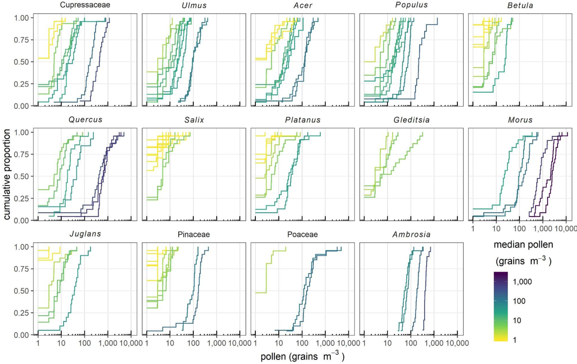
Cumulative distribution of pollen concentrations for each taxon during each sampling event within the 99% pollen season. Each line is a sampling event and each step on the line is a site; the x-axis is the pollen concentration at that site and the y-axis the proportion of sites that had less pollen than that site. Sampling events are color coded by median pollen level (cumulative proportion = 0.5). Steeper lines show more uniform pollen concentrations, and shallower lines more dispersed distributions. Slopes of lines at low concentrations (e.g., < 10 grains m⁻³) may be less meaningful.

Spatial autocorrelation was inconsistent, and nearby sites often had very different pollen concentrations (semivariograms for each taxon and day are provided in SI 4). The strength of autocorrelation varied among taxa and sampling events; the taxa exhibiting the strongest evidence for spatial autocorrelation were Cupressaceae and Quercus.

3.3. Spatio-temporal heterogeneity

For several taxa (e.g., Acer, Ulmus, and Platanus), the site with the highest pollen concentration frequently changed between days, and it was common for a site that had relatively low pollen concentrations on one day to have relatively high pollen concentrations on the subsequent sampling day (SI 5). In contrast, for Cupressaceae, Morus, and Ambrosia, some sites tended to have consistently high pollen concentrations and other sites tended to have consistently low pollen concentrations. Example maps of airborne pollen concentrations including relative and absolute pollen concentrations are provided in SI 5.

The Detroit data show the extent to which pollen concentrations at a single location predict pollen concentrations at other sites. Figure 4 is a scatter plot of all observations from each unique pair of sites. Stronger associations between sites are shown by observations closer to the 1:1 line and by narrower prediction intervals (dashed lines). For example, if 100 pollen grains m⁻³ were observed at one site, the 95% predicted interval at other sites were 4 – 1087 pollen grains m⁻³ for Quercus and 45 – 312 pollen grains m⁻³ for Ambrosia. Model fits as R² ranged from 0.03 (Salix) to 0.85 (Pinaceae and Poaceae); the average R² across tree taxa was 0.37. Analyses using the 95% and 100% pollen season definition, give an average R² of 0.27 and 0.46 respectively. Across the entire season, the 95% predicted intervals often spanned two orders of magnitude.

Figure 4:

Comparison of pollen concentrations between sites across the sampling period for the time-series from each unique pair of sites. The number of observations in each bin is indicated by color and the 95% prediction interval (using the linear model and the log transformed data) is shown for each taxon with dashed lines.

4. Discussion

4.1. Urban scale variation of pollen

Other studies have measured pollen concentrations at the urban scale that correspond to qCOD values ranging from 0.21 to 0.57, with an average qCOD of 0.34 (Bricchi et al. 2000; Charalampopoulos et al. 2018; Emberlin and Norris-Hill 1991; Hjort et al. 2015; Katz and Carey 2014; Weinberger et al. 2018; Werchan et al. 2017). Our Detroit data shows considerably higher variability, e.g., qCOD across taxa here averaged 0.63. For focal taxa, qCOD reported elsewhere was generally far lower than reported here, e.g., 0.26 and 0.21 vs 0.46 respectively for Quercus, 0.42, 0.47, and 0.48 vs 0.87 for Platanus, 0.35 and 0.22 vs 0.83 for Betula, 0.33 and 0.42 vs 0.67 for Acer, 0.26 and 0.21, and 0.42 vs 0.48 for Poaceae, 0.09 vs 0.57 for Cupressaceae, 0.42 vs 0.80 for Pinaceae, 0.29 vs 0.54 for Populus, 0.14 vs 0.42 for Morus, and 0.51 vs 0.52 for Ulmus. Here, qCOD for Ambrosia was 0.18; in a previous study we conducted in Detroit qCOD for Ambrosia was 0.42 but in that study, a portion of samplers were deliberately placed near Ambrosia patches. Potential causes for the relatively higher spatial variation reported here are described below. These results provide strong evidence that pollen concentrations measured at one location are not an effective proxy for concentrations elsewhere within a city or region. This is corroborated by the sharp pollen concentration gradients associated with individual trees at distances of ~100 m in Worcester, UK (Adams-Groom et al. 2017) to hundreds of meters in Perugia, Italy (Bricchi et al. 2000), and from data from a similar study in Toronto, Canada (Lavigne et al., manuscript in prep).

The higher degree of spatial variability reported here than elsewhere may be due to methodological differences. First, we used a daily time-step while the comparison studies used weekly or seasonal time-steps that would tend to miss variability caused by peak flowering occurring on different days within the study area. Second, we sampled at 1.5 m height; in comparison, the recommended height for (permanent) pollen monitoring stations is 5 – 15 m in the United States and 15 – 20 m in Europe. Pollen concentrations near the ground are generally more variable than concentrations measured at greater heights (Rojo et al. 2019; Soldevilla et al. 1995; Spieksma et al. 2000), and can display differences in diurnal timing (Fernández-Rodríguez et al. 2014b), but 1.5 m is approximately breathing height. Several other studies of spatial variation in airborne pollen have also sampled near the ground (Charalampopoulos et al. 2018; Hjort et al. 2015; Ishibashi et al. 2008; Katz et al. 2019; Katz and Carey 2014; Weinberger et al. 2018; Werchan et al. 2017). While many studies that sampled at only a few locations have sampled at elevated heights (Fernández-Rodríguez et al. 2014a; Weinberger et al. 2015), we are only aware of one study that sampled at many locations at elevated heights (Emberlin and Norris-Hill 1991). Furthermore, truncating the time period of an analysis can change how well one site predicts another, e.g., including the periods at the start and end of the pollen season when pollen concentrations were near zero resulted in stronger correlations between sites. In other words, a single station is better at indicating whether the city is in the main pollen season than it is for predicting daily concentrations at other locations during the main pollen season.

4.2. Causes of variation

The spatial variability of pollen concentrations at the urban scale can result from several factors, including spatial variation in plant composition and abundance, the time of flowering and pollen release, and meteorological influences on pollen release and dispersal. Spatial variability in plant composition has been shown to affect pollen concentrations at distances from 100 m (Werchan et al. 2017) to 200 m (Charalampopoulos et al. 2018); the effects of plant composition at larger scales is seldom tested. More comprehensive linkages between plant composition and spatial variability is limited by information on plant location; only a single study had locations of all intra-municipal sources (Bricchi et al. 2000). Other surrogates for plant composition and abundance, including total tree cover (Weinberger et al. 2018), land use type (Hjort et al. 2015), and habitat type availability (Katz and Carey 2014) also have been used to predict airborne pollen. However, urban plant composition results from several complex mechanisms (Roman et al. 2018), limiting the generalizability of indirect proxies for plant abundance. Plant composition within genera can also affect variation in pollen concentrations (Brennan et al. 2019); while pollen of congeneric plants are lumped together during identification they can have distinct flowering phenology (e.g., distinct peaks in Acer pollen could potentially be caused by Acer saccharinum and A. negundo, which we have observed flowering several weeks apart in this area, Katz unpublished data).

Differences in flowering phenology cause lags and leads in pollen concentrations at different sites leading to spatial variability. In the spring of 2017, we monitored flowering phenology of Quercus and Morus trees in Detroit, and found substantial variation in the timing of flowering within the city, which was very well explained by spatial differences in average land surface temperature during February (Katz et al. 2019). These differences in flowering time within the city explained 46% and 70% of the variation in relative pollen levels for Quercus and Morus, respectively. It is plausible that the phenological differences between sites could flip their relative pollen concentrations even on time scales of days (e.g., the 3 or 4 day sampling interval used here). The range of average February temperatures within Detroit (6 °C) is similar to that in other epidemiological studies (average of 5 °C), so phenology is likely to be a principal cause of spatio-temporal variation elsewhere too (Katz et al. 2019).

Meteorological variables can affect pollen release and dispersal, including wind speed, wind direction, and turbulence (Auer et al. 2016; Huang et al. 2015; Klein et al. 2003; Kuparinen 2006). Wind direction will influence the direction of dispersal, and higher wind speeds can increase the distance pollen will travel. Temperature (as discussed) and humidity can affect the timing of pollen release (Martin et al. 2010). These meteorological variables can vary considerably over time and space, potentially causing variation at both local and regional scales. For example, winds could transport air masses from areas with high pollen production on one day; the next day may bring air masses from areas with low pollen production (Hernández-Ceballos et al. 2011; Maya-Manzano et al. 2017). Physical structures such as buildings and tree cover can affect wind patterns and therefore pollen concentrations (Auer et al. 2016). Taxon related differences in spatial variability of pollen could also be caused by pollen release height (Klein et al. 2003), the relative contributions of local vs. regional sources (Hernández-Ceballos et al. 2011), or pollen settling rates (Borrell 2012). Quantitative analyses of the relative contributions of these processes to the variability observed in this study are beyond the present scope, but these data are useful for hypothesis generation. For example, the greater spatial variability seen for Gleditsia tricanthos could hypothetically be driven by its relatively large pollen size (~37 μ), which could result in faster settling rates (Borrell 2012). In another example, the high spatial variability of Betula could hypothetically be due to its relative infrequency in the landscape; sites with higher pollen concentrations may simply have been near source trees. Knowledge of many taxon-specific processes, from plant location and phenology to meteorology and pollen traits, are required to understand the spatio-temporal patterns of pollen observed here and to predict them in other cities. Knowing the circumstances in which a monitoring station is or is not expected to be representative of its area would be useful for both researchers and the public.

4.3. Implications for epidemiological investigations

Epidemiological studies using longitudinal designs may be robust to spatial variation if pollutant concentrations fluctuate in unison within the study area (Wilson et al. 2005). However, the Detroit data show that pollen levels did not increase (or decrease) by the same amount across the sites, or even necessarily change in the same direction. Conducting analyses on a weekly basis (Qin et al. 2013; Werchan et al. 2017, 2018) in which a greater portion of the study area would attain peak pollen levels together, instead of a daily time step, may prevent a false level of precision in pollen concentrations.

The extensive spatial and spatio-temporal variation found in this study suggests that the use of a single monitoring station can result in considerable measurement error in epidemiological analyses that use a daily time step; such errors can lead to incorrect conclusions. However, the variability in pollen levels must be considered with respect to levels that may cause symptoms and adverse health effects. Despite longstanding study of the relationship between pollen concentrations and allergic responses Frenz 2001), population-level responses to pollen vary considerably between epidemiological studies (e.g., Darrow et al., 2012; Erbas et al., 2012; Ito et al., 2015; Sun et al., 2016), so the exact effect of the potential misclassification documented here is unknown. Still, these studies at the population level, as well as studies at the individual level (Frenz 2001), suggest that responses to pollen are continuous and do not saturate at high pollen concentrations, thus misclassification is expected to be important across a broad range of pollen concentrations.

4.4. Implications for pollen monitoring

For many air pollutants, a single monitor does not provide sufficient exposure information and alternate approaches are required (Dionisio et al. 2016). The variability observed in Detroit suggests that any single monitoring station, even if located at NAB or EAN recommended height, will not represent near-ground pollen concentrations across an urban area. Additionally, if the pollen monitoring station is located away from population centers, then it may provide incorrect exposure estimates due to differences in the timing of pollen release (Katz et al. 2019). One approach for reducing exposure misclassification is to monitor pollen at multiple locations within a city (e.g., Werchan et al., 2018). However, large differences in pollen concentrations were frequently observed at nearby sites in Detroit and elsewhere (Adams-Groom et al. 2017; Bricchi et al. 2000), suggesting that even dense sampling networks will only partially explain pollen concentrations.

Mechanistic models of pollen concentrations offer a promising approach to improving urban scale predictions of pollen concentrations. A major barrier has been a lack of comprehensive maps of urban plants. While such maps are rare, they are becoming feasible for trees due to advances in remote sensing (Wang et al. 2019) and are already fully operational for grass (Skjøth et al. 2013). Taxa with distinct habitat preferences, such as ragweed, can also be mapped and modeled effectively (Katz and Batterman 2019). Plant maps could be combined with pollen production estimates (Katz et al. manuscript in press in Aerobiologia, DOI : 10.1007/s10453-020-09638-8, AERO-D-19-00114R1), phenology models, and atmospheric dispersion models to more accurately predict and forecast airborne pollen concentrations.

4.4. Sampler variability

Measurements reported here were collected over 24 hour periods and escape the limitations imposed by sequential sampling and gravitational sampling. Wind speed can affect sampler efficiency, but effects are expected to be <20% for speeds commonly observed during sampling (Frenz 2000). Rotorod samplers are one of two sampler types widely used by the National Allergy Bureau pollen monitoring network and in epidemiological analyses. Differences between rotorods and the other most commonly used active sampler, Burkards, are generally small for pollen (< 20% difference in means), although differences do depend on wind speed and particle size (Di-Giovanni 1998; Frenz 2000; Miki et al. 2017). It should also be noted that pollen concentrations observed in Detroit are generally in the same range as concentrations reported in epidemiological analyses (e.g., Darrow et al., 2012; Guilbert et al., 2016; Ito et al., 2015; Sun et al., 2016), with the exception of Ambrosia concentrations, which were substantially higher at 709 pollen grains m⁻³ (maximum recorded), compared to ~60 pollen grains m⁻³ (Darrow et al. 2012), ~50 pollen grains m⁻³ (Gleason et al. 2014), and <30 pollen grains m⁻³ (Sun et al. 2016).

4.5. Study limitations

Spatio-temporal variation in pollen concentrations was evaluated in only one city, and results may vary between cities. Sampling was conducted in a single year, but the quantity of pollen produced and the timing of release could vary between years. Urban plant distributions are determined by complex processes that are expected to vary between cities, likely resulting in distinct spatial patterns of pollen release in each city. Still, urban vegetation is generally becoming more similar among cities (Groffman et al. 2014), and tree composition in Detroit (as per street tree data) does not appear unusual. Results for ragweed, which thrives in vacant lots and disturbed soils that are common in Detroit, may be less generalizable, although findings for this taxon may still apply to other depopulating cities. Additionally, the results for Ambrosia and Poaceae were based on only four and two sampling events respectively, so results for these taxa should be interpreted with some caution.

5. Conclusion

Based on a comprehensive set of 24-hour measurements of 13 taxa, spatial and spatio-temporal variability of airborne pollen concentrations was high in Detroit. This novel dataset demonstrates that pollen measurements from a single site are unlikely to represent exposure over an urban area. The amount of variability varied between taxa, and pollen concentrations were generally more homogenous on high pollen days. The spatio-temporal variation of pollen concentrations can represent a potentially important source of exposure measurement error in epidemiological analyses, particularly for studies using a 24-hr time step. Such errors might be reduced by using longer time steps (e.g., 1 week), or by applying new methods that model pollen concentrations over space and time.

References

- Adams-Groom B, Skjoth CA, Baker M, & Welch TE (2017). Modelled and observed surface soil pollen deposition distance curves for isolated trees of Carpinus betulus, Cedrus atlantica, Juglans nigra and Platanus acerifolia. Aerobiologia, 33(3), 1–10. doi: 10.1007/s10453-017-9479-128255194 [DOI] [Google Scholar]
- Auer C, Meyer T, & Sagun V (2016). Reducing Pollen Dispersal using Forest Windbreaks. Plant Science Articles. [Google Scholar]
- Blaiss MS, Hammerby E, Robinson S, Kennedy-Martin T, & Buchs S (2018). The burden of allergic rhinitis and allergic rhinoconjunctivitis on adolescents: A literature review. Annals of Allergy, Asthma and Immunology, 121(1), 43–52.e3. doi: 10.1016/j.anai.2018.03.028 [DOI] [PubMed] [Google Scholar]
- Bonett DG (2006). Confidence interval for a coefficient of quartile variation. Computational Statistics and Data Analysis, 50(11), 2953–2957. doi: 10.1016/j.csda.2005.05.007 [DOI] [Google Scholar]
- Borrell JS (2012). Rapid assessment protocol for pollen settling velocity: Implications for habitat fragmentation. Bioscience Horizons, 5, 1–9. doi: 10.1093/biohorizons/hzs002 [DOI] [Google Scholar]
- Bousquet J, Khaltaev N, Cruz AA, Denburg J, Fokkens WJ, Togias A, et al. (2008). Allergic Rhinitis and its Impact on Asthma (ARIA) 2008 update (in collaboration with the World Health Organization, GA2LEN and AllerGen). Allergy: European Journal of Allergy and Clinical Immunology, 63(SUPPL. 86), 8–160. doi: 10.1111/j.1398-9995.2007.01620.x [DOI] [PubMed] [Google Scholar]
- Brennan GL, Potter C, de Vere N, Griffith GW, Skjøth CA, Osborne NJ, et al. (2019). Temperate airborne grass pollen defined by spatio-temporal shifts in community composition. Nature Ecology and Evolution, 3(May). doi: 10.1038/s41559-019-0849-7 [DOI] [PubMed] [Google Scholar]
- Bricchi E, Frenguelli G, & Mincigrucci G (2000). Experimental results about Platanus pollen deposition. Aerobiologia, 16, 347–352. http://link.springer.com/article/10.1023/A:1026701028901. Accessed 13 December 2013 [Google Scholar]
- Cardell LO, Olsson P, Andersson M, Welin KO, Svensson J, Tennvall GR, & Hellgren J (2016). TOTALL: High cost of allergic rhinitis - a national Swedish population-based questionnaire study. Primary Care Respiratory Medicine, 26(15082), 1–5. doi: 10.1038/npjpcrm.2015.82 [DOI] [PMC free article] [PubMed] [Google Scholar]
- Charalampopoulos A, Lazarina M, Tsiripidis I, & Vokou D (2018). Quantifying the relationship between airborne pollen and vegetation in the urban environment. Aerobiologia, 34(3), 1–16. doi: 10.1007/s10453-018-9513-y [DOI] [Google Scholar]
- D’Amato G, Cecchi L, Bonini S, Nunes C, Annesi-Maesano I, Behrendt H, et al. (2007). Allergenic pollen and pollen allergy in Europe. Allergy, 62(9), 976–90. doi: 10.1111/j.1398-9995.2007.01393.x [DOI] [PubMed] [Google Scholar]
- Darrow L. a, Hess J, Rogers C. a, Tolbert PE, Klein M, & Sarnat SE (2012). Ambient pollen concentrations and emergency department visits for asthma and wheeze. The Journal of allergy and clinical immunology, 130(3), 630–638.e4. doi: 10.1016/j.jaci.2012.06.020 [DOI] [PMC free article] [PubMed] [Google Scholar]
- Di-Giovanni F (1998). A review of the sampling efficiency of rotating-arm impactors used in aerobiological studies. Grana, 37(3), 164–171. doi: 10.1080/00173139809362661 [DOI] [Google Scholar]
- Dionisio KL, Baxter LK, Burke J, & Özkaynak H (2016). The importance of the exposure metric in air pollution epidemiology studies: When does it matter, and why? Air Quality, Atmosphere and Health, 9(5), 495–502. doi: 10.1007/s11869-015-0356-1 [DOI] [Google Scholar]
- Emberlin J, & Norris-Hill J (1991). Spatial variation of pollen deposition in North London. Grana, 30(1), 190–195. doi: 10.1080/00173139109427798 [DOI] [Google Scholar]
- Endsley KA, Brown DG, & Bruch E (2018). Housing Market Activity is Associated with Disparities in Urban and Metropolitan Vegetation. Ecosystems, 21(8), 1–15. doi: 10.1007/s10021-018-0242-431156332 [DOI] [Google Scholar]
- Erbas B, Akram M, Dharmage SC, Tham R, Dennekamp M, Newbigin E, et al. (2012). The role of seasonal grass pollen on childhood asthma emergency department presentations. Clinical and Experimental Allergy, 42(5), 799–805. doi: 10.1111/j.1365-2222.2012.03995.x [DOI] [PubMed] [Google Scholar]
- Fernández-Rodríguez S, Tormo-Molina R, Maya-Manzano JM, Silva-Palacios I, & Gonzalo-Garijo Á (2014a). Comparative study of the effect of distance on the daily and hourly pollen counts in a city in the south-western Iberian Peninsula. Aerobiologia, 30(2), 173–187. doi: 10.1007/s10453-013-9316-0 [DOI] [Google Scholar]
- Fernández-Rodríguez S, Tormo-Molina R, Maya-Manzano JM, Silva-Palacios I, & Gonzalo-Garijo Á (2014b). A comparative study on the effects of altitude on daily and hourly airborne pollen counts. Aerobiologia, 30(3), 257–268. doi: 10.1007/s10453-014-9325-7 [DOI] [Google Scholar]
- Frenz DA (2001). Interpreting atmospheric pollen counts for use in clinical allergy: Allergic symptomology. Annals of Allergy, Asthma and Immunology, 86(2), 150–158. doi: 10.1016/S1081-1206(10)62683-X [DOI] [PubMed] [Google Scholar]
- Frenz David A. (2000). The effect of windspeed on pollen and spore counts collected with the Rotorod Sampler and Burkard spore trap. Annals of Allergy, Asthma and Immunology, 85(5), 392–394. doi: 10.1016/S1081-1206(10)62553-7 [DOI] [PubMed] [Google Scholar]
- Frenz DA, Scamehorn RT, Hokanson JM, & Murray LW (1996). A brief method for analyzing rotorod samples for pollen content. Aerobiologia, 12, 51–54. [Google Scholar]
- Gleason JA, Bielory L, & Fagliano JA (2014). Associations between ozone, PM2.5, and four pollen types on emergency department pediatric asthma events during the warm season in New Jersey: A case-crossover study. Environmental Research, 132, 421–429. doi: 10.1016/j.envres.2014.03.035 [DOI] [PubMed] [Google Scholar]
- Gräler B, Pebesma E, & Heuvelink G (2016). Spatio-Temporal Interpolation using gstat. The R Journal, 8(1), 204–218. http://journal.r-project.org/archive/2016-1/na-pebesma-heuvelink.pdf [Google Scholar]
- Groffman PM, Cavender-Bares J, Bettez ND, Grove JM, Hall SJ, Heffernan JB, et al. (2014). Ecological homogenization of urban USA. Frontiers in Ecology and the Environment, 12(1), 74–81. doi: 10.1890/120374 [DOI] [Google Scholar]
- Guilbert A, Simons K, Hoebeke L, Packeu A, Hendrickx M, De Cremer K, et al. (2016). Short-term effect of pollen and spore exposure on allergy morbidity in the Brussels-Capital Region. EcoHealth, 13(2), 303–315. doi: 10.1007/s10393-016-1124-x [DOI] [PMC free article] [PubMed] [Google Scholar]
- Hepworth W., Vinay P, & Zenger V (1983). Airborne and allergenic pollen of North America Airborne and Allergenic Pollen of North America. Baltimore: Johns Hopkins University Press. [Google Scholar]
- Hernández-Ceballos MA, García-Mozo H, Adame JA, Domínguez-Vilches E, Bolívar JP, De La Morena BA, et al. (2011). Determination of potential sources of Quercus airborne pollen in Cordoba city (southern Spain) using back-trajectory analysis. Aerobiologia, 27(3), 261–276. doi: 10.1007/s10453-011-9195-1 [DOI] [Google Scholar]
- Hjort J, Hugg TT, Antikainen H, Rusanen J, Sofiev M, Jaakkola MS, & Jaakkola JJK (2015). Fine-scale exposure to allergenic pollen in the urban environment: Evaluation of land use regression approach. Environmental Health Perspectives, 124(5), 619–626. doi: 10.1289/ehp.1509761 [DOI] [PMC free article] [PubMed] [Google Scholar]
- Huang H, Ye R, Qi M, Li X, Miller DR, Stewart CN, et al. (2015). Wind-mediated horseweed (Conyza canadensis) gene flow: Pollen emission, dispersion, and deposition. Ecology and Evolution, 5(13), 2646–2658. doi: 10.1002/ece3.1540 [DOI] [PMC free article] [PubMed] [Google Scholar]
- Hugg T, & Rantio-Lehtimäki A (2007). Indoor and outdoor pollen concentrations in private and public spaces during the Betula pollen season. Aerobiologia, 23(2), 119–129. doi: 10.1007/s10453-007-9057-z [DOI] [Google Scholar]
- Ishibashi Y, Ohno H, Oh-ishi S, Matsuoka T, Kizaki T, & Yoshizumi K (2008). Characterization of pollen dispersion in the neighborhood of Tokyo, Japan in the spring of 2005 and 2006. International Journal of Environmental Research and Public Health, 5(1), 76–85. doi: 10.3390/ijerph5020076 [DOI] [PMC free article] [PubMed] [Google Scholar]
- Ito K, Weinberger KR, Robinson GS, Sheffield PE, Lall R, Mathes R, et al. (2015). The associations between daily spring pollen counts, over-the-counter allergy medication sales, and asthma syndrome emergency department visits in New York City, 2002–2012. Environmental Health, 14(1), 71. doi: 10.1186/s12940-015-0057-0 [DOI] [PMC free article] [PubMed] [Google Scholar]
- Kahle D, & Wickham H (2013). ggmap: Spatial Visualization with ggplot2. The R Journal, 5(1), 144–161. http://journal.r-project.org/archive/2013-1/kahle-wickham.pdf [Google Scholar]
- Katz DSW, & Batterman SA (2019). Allergenic pollen production across a large city for common ragweed (Ambrosia artemisiifolia). Landscape and Urban Planning, 190(March), 103615. doi: 10.1016/j.landurbplan.2019.103615 [DOI] [PMC free article] [PubMed] [Google Scholar]
- Katz DSW, & Carey TS (2014). Heterogeneity in ragweed pollen exposure is determined by plant composition at small spatial scales. Science of The Total Environment, 485, 435–440. doi: 10.1016/j.scitotenv.2014.03.099 [DOI] [PubMed] [Google Scholar]
- Katz DSW, Dzul A, Kendel A, & Batterman SA (2019). Effect of intra-urban temperature variation on tree flowering phenology, airborne pollen, and measurement error in epidemiological studies of allergenic pollen. Science of The Total Environment, 653, 1213–1222. doi: 10.1016/j.scitotenv.2018.11.020 [DOI] [PMC free article] [PubMed] [Google Scholar]
- Klein E, Lavigne C, Foueillassar X, Gouyon P, & Laredo C (2003). Corn pollen dispersal: quasi-mechanistic models and field experiments. Ecological Monographs, 73(1), 131–150. http://www.esajournals.org/doi/abs/10.1890/0012-9615(2003)073%5B0131:CPDQMM%5D2.0.CO%3B2 [Google Scholar]
- Kuparinen A (2006). Mechanistic models for wind dispersal. Trends in plant science, 11(6), 296–301. doi: 10.1016/j.tplants.2006.04.006 [DOI] [PubMed] [Google Scholar]
- La Rosa M, Lionetti E, Reibaldi M, Russo A, Longo A, Leonardi S, et al. (2013). Allergic conjunctivitis: a comprehensive review of the literature. Italian Journal of Pediatrics, 39, 18. doi: 10.1186/1824-7288-39-18 [DOI] [PMC free article] [PubMed] [Google Scholar]
- Levetin E (2004). Methods for aeroallergen sampling. Current Allergy and Asthma Reports, 4(5), 376–383. doi: 10.1007/s11882-004-0088-z [DOI] [PubMed] [Google Scholar]
- Linneberg A, Henrik Nielsen N, Frølund L, Madsen F, Dirksen A, & Jørgensen T (2002). The link between allergic rhinitis and allergic asthma: A prospective population-based study. The Copenhagen Allergy Study. Allergy: European Journal of Allergy and Clinical Immunology, 57(11), 1048–1052. doi: 10.1034/j.1398-9995.2002.23664.x [DOI] [PubMed] [Google Scholar]
- Martin MD, Chamecki M, & Brush GS (2010). Anthesis synchronization and floral morphology determine diurnal patterns of ragweed pollen dispersal. Agricultural and Forest Meteorology, 150(9), 1307–1317. doi: 10.1016/j.agrformet.2010.06.001 [DOI] [Google Scholar]
- Maya-Manzano JM, Sadyś M, Tormo-Molina R, Fernández-Rodríguez S, Oteros J, Silva-Palacios I, & Gonzalo-Garijo A (2017). Relationships between airborne pollen grains, wind direction and land cover using GIS and circular statistics. Science of The Total Environment. doi: 10.1016/j.scitotenv.2017.01.085 [DOI] [PubMed] [Google Scholar]
- Meltzer EO (2016). Allergic rhinitis: Burden of illness, quality of life, comorbidities, and control. Immunology and Allergy Clinics of North America, 36(2), 235–248. doi: 10.1016/j.iac.2015.12.002 [DOI] [PubMed] [Google Scholar]
- Meltzer EO, Blaiss MS, Derebery MJ, Mahr TA, Gordon BR, Sheth KK, et al. (2009). Burden of allergic rhinitis: Results from the Pediatric Allergies in America survey. Journal of Allergy and Clinical Immunology, 124(3 SUPPL. 1), 43–70. doi: 10.1016/j.jaci.2009.05.013 [DOI] [PubMed] [Google Scholar]
- Miki K, Kawashima S, Fujita T, Nakamura K, & Clot B (2017). Effect of micro-scale wind on the measurement of airborne pollen concentrations using volumetric methods on a building rooftop. Atmospheric Environment, 158, 1–10. doi: 10.1016/j.atmosenv.2017.03.015 [DOI] [Google Scholar]
- Mims JW (2014). Epidemiology of allergic rhinitis. International Forum of Allergy and Rhinology, 4(SUPPL.2), 18–20. doi: 10.1002/alr.21385 [DOI] [PubMed] [Google Scholar]
- Nathan R (2007). The burden of allergic rhinitis. Allergy and Asthma Proceedings, 28(1), 3–9. doi: 10.2500/aap.2007.28.2934 [DOI] [PubMed] [Google Scholar]
- Osborne NJ, Alcock I, Wheeler BW, Hajat S, Sarran C, Clewlow Y, et al. (2017). Pollen exposure and hospitalization due to asthma exacerbations: daily time series in a European city. International Journal of Biometeorology, 61(10), 1837–1848. doi: 10.1007/s00484-017-1369-2 [DOI] [PMC free article] [PubMed] [Google Scholar]
- Peel RG, Kennedy R, Smith M, & Hertel O (2014). Do urban canyons influence street level grass pollen concentrations? International Journal of Biometeorology, 58(6), 1317–1325. doi: 10.1007/s00484-013-0728-x [DOI] [PubMed] [Google Scholar]
- Qin P, Waltoft BL, Mortensen PB, & Postolache TT (2013). Suicide risk in relation to air pollen counts: a study based on data from Danish registers. BMJ open, 3(5), e002462. doi: 10.1136/bmjopen-2012-002462 [DOI] [PMC free article] [PubMed] [Google Scholar]
- R Core Team. (2018). R: A language and environment for statistical computing. Vienna, Austria. doi: 10.1145/192593.192639 [DOI] [Google Scholar]
- Rojo J, Oteros J, Pérez-badia R, Cervigón P, Ferencova Z, Gutiérrez-bustillo AM, et al. (2019). Near-ground effect of height on pollen exposure. Environmental Research. doi: 10.1016/j.envres.2019.04.027 [DOI] [PubMed] [Google Scholar]
- Roman LA, Pearsall H, Eisenman TS, Conway TM, Fahey RT, Landry S, et al. (2018). Human and biophysical legacies shape contemporary urban forests: A literature synthesis. Urban Forestry and Urban Greening, 31(December 2017), 157–168. doi: 10.1016/j.ufug.2018.03.004 [DOI] [Google Scholar]
- Sakata S, Konishi S, Ng CFS, Kishikawa R, & Watanabe C (2017). Association of Asian Dust with daily medical consultations for pollinosis in Fukuoka City, Japan. Environmental Health and Preventive Medicine, 22(1), 25. doi: 10.1186/s12199-017-0623-x [DOI] [PMC free article] [PubMed] [Google Scholar]
- Salo P, Calatroni A, Gergen P, Hoppin J, Sever M, Jaramillo R, et al. (2011). Allergy-related outcomes in relation to serum IgE: Results from the National Health and Nutrition Examination Survey 2005–2006. Journal of Allergy and Clinical Immunology, 127(5), 1226–1235. doi: 10.1016/j.jaci.2010.12.1106.Allergy-related [DOI] [PMC free article] [PubMed] [Google Scholar]
- Skjøth C. a., Ørby PV, Becker T, Geels C, Schlünssen V, Sigsgaard T, et al. (2013). Identifying urban sources as cause of elevated grass pollen concentrations using GIS and remote sensing. Biogeosciences, 10(1), 541–554. doi: 10.5194/bg-10-541-2013 [DOI] [Google Scholar]
- Smith G (1984). Sampling and identifying allergenic pollens and moulds. San Antonio, Texas: Blewstone Press. [Google Scholar]
- Soldevilla CG, Alcfizar-Teno P, & Dominguez-Vilches E (1995). Airborne pollen grain concentrations at two different heights. Aerobiologia Aerobiologia Internalional Journal of Aerobiology, 11, 105–109. doi: 10.1007/BF02738275 [DOI] [Google Scholar]
- Spieksma FTM, Van Noort P, & Nikkels H (2000). Influence of nearby stands of Artemisia on street-level versus roof-top-level ratio’s of airborne pollen quantities. Aerobiologia, 16(1), 21–24. doi: 10.1023/A:1007618017071 [DOI] [Google Scholar]
- Sun X, Waller A, Yeatts KB, & Thie L (2016). Pollen concentration and asthma exacerbations in Wake County, North Carolina, 2006–2012. Science of the Total Environment, 544, 185–191. doi: 10.1016/j.scitotenv.2015.11.100 [DOI] [PubMed] [Google Scholar]
- Wang J, Qi M, Huang H, Ye R, Li X, & Neal Stewart C (2017). Atmospheric pollen dispersion from herbicide-resistant horseweed (Conyza canadensis L.). Aerobiologia, 33(3), 393–406. doi: 10.1007/s10453-017-9477-3 [DOI] [Google Scholar]
- Wang K, Wang T, & Liu X (2019). A review: individual tree species classification using integrated airborne LiDAR and optical imagery with a focus on the urban environment. Forests, 10(1), 1–18. doi: 10.3390/f10010001 [DOI] [Google Scholar]
- Weinberger KR, Kinney PL, & Lovasi GS (2015). A review of spatial variation of allergenic tree pollen within cities. Arboriculture & Urban Forestry, 41(2), 57–68. [Google Scholar]
- Weinberger KR, Kinney PL, Robinson GS, Sheehan D, Kheirbek I, Matte TD, & Lovasi GS (2018). Levels and determinants of tree pollen in New York City. Journal of Exposure Science and Environmental Epidemiology, 28(2), 119–124. doi: 10.1038/jes.2016.72 [DOI] [PMC free article] [PubMed] [Google Scholar]
- Werchan B, Werchan M, Mücke H-G, Gauger U, Simoleit A, Zuberbier T, & Bergmann K-C (2017). Spatial distribution of allergenic pollen through a large metropolitan area. Environmental Monitoring and Assessment, 189(4), 169. doi: 10.1007/s10661-017-5876-8 [DOI] [PubMed] [Google Scholar]
- Werchan B, Werchan M, Mücke HG, & Bergmann KC (2018). Spatial distribution of pollen-induced symptoms within a large metropolitan area—Berlin, Germany. Aerobiologia, 34(4), 539–556. doi: 10.1007/s10453-018-9529-3 [DOI] [Google Scholar]
- Wickham H (2009). ggplot2: elegant graphics for data analysis. New York, NY: Springer; http://had.co.nz/ggplot2/book [Google Scholar]
- Wilson JG, Kingham S, Pearce J, & Sturman AP (2005). A review of intraurban variations in particulate air pollution: Implications for epidemiological research. Atmospheric Environment, 39(34), 6444–6462. doi: 10.1016/j.atmosenv.2005.07.030 [DOI] [Google Scholar]
Associated Data
This section collects any data citations, data availability statements, or supplementary materials included in this article.