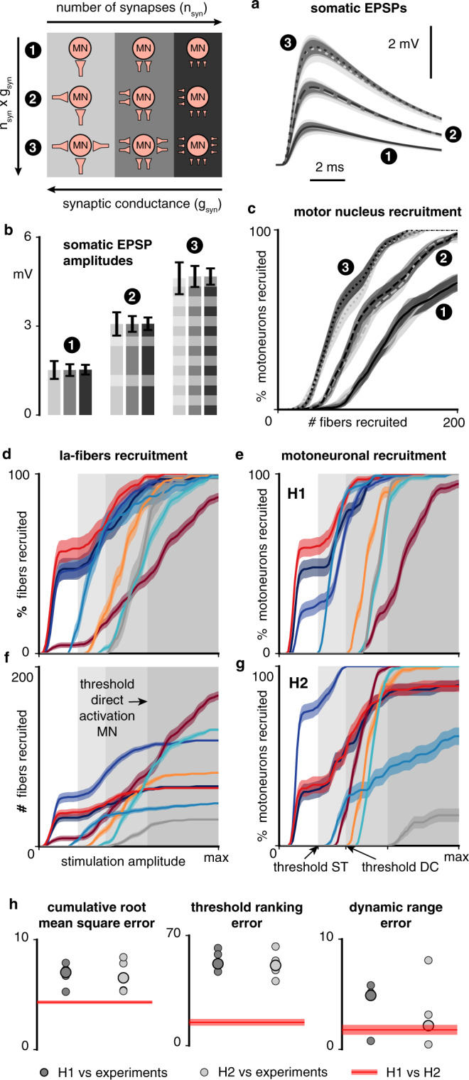
Fig. 6. Computational analysis of the Ia-mediated recruitment of motoneurons.

a Time course of the somatic excitatory post-synaptic potential (EPSP) induced in a motoneuron model by various populations of synapses, for different population sizes nsyn and synaptic conductances gsyn. Lines (solid, dashed and dotted) and filled areas represent the mean and standard deviation of the EPSPs obtained with 100 random synapse populations for each condition (9 conditions in total, see legend in the top left corner and “Methods”). b Maximal amplitudes of the EPSPs of (a). Bars and whiskers: mean ± standard deviation computed across the 100 synapse populations for each condition. c Recruitment of a motor nucleus as a function of the number of simultaneously activated fibers innervating this motor nucleus, for different connectivity ratios and synaptic conductances. Higher connectivity ratios are indicated by higher numbers of synapses in the legend. d Recruitment of Ia-fibers of specific muscles following electrical stimulation from a lateral contact at the C6 spinal level (Fig. 2a). e Monosynaptic recruitment of motoneurons resulting from the Ia-fiber recruitment shown in (d) using muscle-specific synaptic conductances (hypothesis H1, see Supplementary Table 1). f Same Ia-fiber recruitment as in (d) but represented in absolute numbers of recruited fibers. g Same as (e) but using a uniform synaptic conductance of 7.625 pS (hypothesis H2). h Comparison between experimental muscular recruitment curves and simulated motoneuronal recruitment curves with H1 or H2 (see “Methods”). Each bullet represents the comparison score for one animal (5 animals in total). Circled bullets indicate the medians across the 5 animals. Simulated Ia-fiber and motoneuron recruitment curves (c–g): curves are made of 80 data points (except for c, 40 data points) consisting in the mean and standard deviation of the recruitment computed across 10,000 bootstrapped populations (see “Methods”). Lines and filled areas represent the moving average over three consecutive data points.
