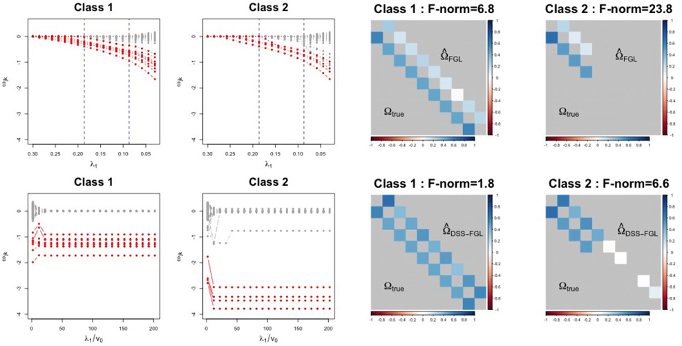
Figure 1.

The solution paths and estimated precision matrices of FGL (upper row) and DSS-FGL (lower row). The red nodes correspond to true edges and the gray nodes correspond to 0’s. The two vertical lines in the FGL solution path indicate the model that best matches the true sparsity (left) and the model with the lowest AIC (right). The block containing the edges is plotted for the estimated values (upper triangular) against the truth (lower triangular). The model that best matches the true graphs is plotted for FGL. The off-diagonal values are rescaled and negated to partial correlations, and 0’s are colored with light gray background for easier visual comparison. The bias of the estimated precision matrix as measured by the Frobenius norm, $\Vert {\widehat{\Omega }}_g-{\Omega }_g{\Vert }_F$, is also printed in the captions.