Hybrid method for representing ions in implicit solvation calculations

Graphical abstract

Abstract

Fast and accurate calculations of the electrostatic features of highly charged biomolecules such as DNA, RNA, and highly charged proteins are crucial and challenging tasks. Traditional implicit solvent methods calculate the electrostatic features quickly, but these methods are not able to balance the high net biomolecular charges effectively. Explicit solvent methods add unbalanced ions to neutralize the highly charged biomolecules in molecular dynamic simulations, which require more expensive computing resources. Here we report developing a novel method, Hybridizing Ions Treatment (HIT), which hybridizes the implicit solvent method with an explicit method to realistically calculate the electrostatic potential for highly charged biomolecules. HIT utilizes the ionic distribution from an explicit method to predict the bound ions. The bound ions are then added in the implicit solvent method to perform the electrostatic potential calculations. In this study, two training sets were developed to optimize parameters for HIT. The performance on the testing set demonstrates that HIT significantly improves the electrostatic calculations. Results on molecular motors myosin and kinesin reveal some mechanisms and explain some previous experimental findings. HIT can be widely used to study highly charged biomolecules, including DNA, RNA, molecular motors, and other highly charged biomolecules. The HIT package is available at http://compbio.utep.edu/static/downloads/download_hit.zip.

1. Introduction

In computational biology, electrostatic calculation of biomolecules is fundamental and challenging. The electrostatic interactions play significant roles in protein folding [1], protein stability [2], [3], protein–protein interactions [4], [5], [6], protein-DNA/RNA interactions [7], [8], and many other areas of study. However, in vivo, water, ions, and small biomolecules make the proteinaceous environment extremely complicated for electrostatic calculations. The highly charged biomolecules (including DNAs, RNAs, and motor proteins) utilize ions surrounding their surfaces to balance the net charges so that they can well interact with other molecules. The trapped ions directly affect the electrostatic surfaces, which have significant impacts on the interactions between biomolecules. Currently, two types of models handle the ions and water molecules surrounding biomolecules: implicit solvent models and explicit solvent models. The most popular implicit solvent methods include the Poisson-Boltzmann (PB) model [9] and Generalized Born (GB) model [10]. In implicit solvent models, biomolecular electrostatic features are calculated by treating ions implicitly [9], [11], [12]. Explicit solvent models such as TIP3P and TIP4P, widely used in Molecular Dynamic (MD) simulations, handle ions and molecules explicitly [13]. Explicit solvent models neutralize the highly charged biomolecules by adding unbalanced amounts of positive and negative ions into a system. Implicit models, such as DelPhi [14], [15], are widely used to calculate electrostatic potential, electric field lines and electrostatic surfaces for biomolecules. However, traditional implicit solvent models treat the solvation as neutral with the same amounts of positive and negative ionic charges, which causes bias in the electrostatic calculations of highly charged biomolecules and causes unrealistic interaction analyses. Improving implicit models to handle highly charged biomolecules remains a challenge.

Highly charged biomolecules have been studied for decades for their special functions, such as the motion of motor proteins [16], [17], [18], tRNA binding of ribosomes [19], and roles of cell aging-related proteins [20], [21]. In living cells, binding of oppositely charged ions by proteins is a principal, common phenomenon related to enzyme-activations [22] and conformational changes of proteins [23]. The classic implicit model does not consider those bound ions and thus cannot balance the net charges of the highly charged biomolecules. The loss of bound ions not only unbalances the system’s net charge; it also leads to biased electrostatic calculations surrounding the ionic binding sites. To perform realistic electrostatic calculations of highly charged biomolecules, we developed a novel method, which adds the bound ions explicitly and hybridizes with implicit ions to compensate for the net charges in highly charged biomolecular systems.

The bound ions in binding sites are crucial for electrostatic calculations of highly charged biomolecules. Such bound ions are not represented in the implicit solvent models. Many methods have been developed to predict such bound ions or the corresponding cavities: Variational Implicit-Solvent Model successfully captures the surface of local hydrophobic cavities for ligand-receptor bindings [24], [25], [26]; BION (bound ion prediction method) program [27] implements electrostatic features and geometric information to predict bound ions. Here we report developing a novel algorithm that utilizes information from MD simulations to identify ion binding sites. Explicit solvent models treat ions explicitly in calculations such as MD simulations. Therefore, the trajectories from MD simulations with explicit models contain the dynamic information of the bound ions. However, it is difficult to determine which ions are bound ions based on a single frame from simulations. Combining all frames from a simulation trajectory into an ionic cloud distribution and properly analyzing it may lead to identification of the binding sites and explicit ions addition. In this report, we introduce a novel method that uses the information from the explicit solvation modeled MD simulations to identify binding sites around highly charged biomolecules. Because this method hybridizes the explicit ions on binding sites and implicit solvent models to calculate the electrostatic potentials of the highly charged biomolecules, we named it Hybridizing Ions Treatment (HIT). We tested this method by using NAMD [28] and Delphi to do the explicit solvent simulations and implicit solvent calculations, respectively; HIT significantly improved the performance of pure implicit models on highly charged biomolecules.

The method was optimized against two training sets and applied to a testing set with two biological applications: A cardiac myosin-actin complex with a net charge of −77e and a kinesin-5 (cut7)-αβ-tubulin complex with a net charge of −36e. Both net charges were calculated by pdb2pqr [29]. Myosin is a superfamily of motor proteins known for their role in muscle contraction [30], especially in heart diseases [31], [32], [33]. We studied myosin-actin complex: β cardiac myosin [34] and part of a cardiac actin filament [35]. Usually, an actin filament is assembled by globular-actin (G-actin), tropomyosin (TM), the troponin complex (Tn) [36], and myosin binding protein C (MyBP-C) [37]. In this study, the TM, G-actin and myosin motor domains were assembled and applied for MD simulations and related analysis by HIT. Kinesin [5], [38] is a superfamily of motor proteins moving along microtubules that are crucial for mitosis [39] and were recently identified as an important target for cancer treatment [40]. In our study, the yeast kinesin-5 (cut7) motor domain with an αβ-tubulin heterodimer complex was selected [41]. The success of the testing set revealed that our method could be widely applied to highly charged biomolecules to obtain reliable electrostatic calculations. By taking advantage of explicit and implicit solvent models, this novel approach utilizes a hybrid method to realistically simulate the solution environment surrounding biomolecules, which is a promising direction for simulations of highly charged biomolecules. Such a method advances future drug design, DNA/RNA simulations, protein–protein interactions, and other computational biophysics research fields.

2. Methodology

2.1. Dataset

2.1.1. Training sets

To optimize our program, two training sets were designed to mimic the sodium distribution surrounding biomolecules in saline solution (150 mM NaCl). One training set was generated by a random generation algorithm (Random ions training set); the other was achieved by MD simulation (NAMD training set).

Random ions training set: To model this 150 mM NaCl concentration into the training dataset, 90 randomly generated sodium ions were placed in a 100 Å × 100 Å × 100 Å box (Fig. 1A), which includes 8 bound sodium ions (8/90 < 10% for bigger solvent box). In the generation process, the minimal distance between sodium ions was set as 5 Å due to the exclusion of same charged ions. 82 randomly generated ions represented free ions while the 8 bound ions represented the ions that were trapped on the surface or in the cavities of the biomolecules. After this, the simulation started for 1000 steps. Each step allowed free ions to move anywhere in the box and restrained bound ions in 5 Å × 5 Å × 5 Å cubic binding sites. The frames for every step were saved (Fig. 1A). All 1000 frames were combined into an ionic cloud distribution for further analysis (Figs. 1B and 2C and D), where the binding sites were marked by black circles. This ionic cloud distribution is the Random ions training set NAMD training set: In Visual Molecular Dynamics (VMD) [42], a 100 Å × 100 Å ×100 Å solvated box with 150 mM NaCl was generated, which included 90 sodium ions and 90 chlorine ions. In this model, 8 sodium ions were randomly selected to be restrained, simulating 8 bound ions in 8 binding sites. After that, MD simulation was achieved by 1000 steps minimization and 0.5 ns (2 fs/step) MD simulation. Temperature was set as 300 K, and the pH was set as 7.0. The CHARMM [43] was used for force field, and the periodic boundary conditions were applied to the system. The frames were saved per 100 fs. After simulation, the ionic cloud distribution for all ions were saved as the NAMD training set.

Fig. 1.

Process of generating the training dataset. A: Schematic presentation of 1000 frames of ions; B: Ionic cloud distribution of the combination of 1000 frames from A; binding sites are marked by black circles; C: Cubic partition of the ionic cloud.

Fig. 2.

Myosin-actin complex (A) and Kinesin-tubulin dimer complex (B) and their sodium ionic cloud distribution. In A, blue chain represents cardiac myosin motor domain, yellow chain represents tropomyosin; the others are G-actin. In B, blue chain represents kinesin-5 (cut7) motor domain, red and orange chains represent αβ-tubulin heterodimer. C and D are the sodium ionic cloud distribution of myosin complex (A) and kinesin complex (B) within 10 ns simulation (1000 frames). (For interpretation of the references to color in this figure legend, the reader is referred to the web version of this article.)

2.1.2. Myosin and kinesin testing sets

In myosin testing set, five G-actins, a TM (PDB: 5NOJ), and a β-cardiac myosin motor domain (PDB: 6FSA) were assembled based on the rigor-like state model (PDB: 5JLH) (Fig. 2A). The hydrogen atoms were added by VMD. The myosin-actin complex was immersed in a rectangular solvated box (TIP3P). The net charge of myosin-actin complex model is −77 e. To ensure 150 mM NaCl and to neutralize the system, 570 Na⁺ and 493 Cl^- were added to the system. In NAMD simulations, the pH was set as 7.0 and the temperature was set as 300 K. The CHARMM was used for force field, and the periodic boundary conditions were applied to the system. The number of steps for energy minimization was 20,000, and the MD simulation was run for 10 ns (1 fs/step). After simulation, the sodium ions within 10 Å from proteins in 2000 frames (5000 steps/frame) were assembled as an ionic cloud distribution in the myosin testing set (Fig. 2C).

Similarly, a complex formed by an αβ-tubulin heterodimer and a kinesin motor domain (kinesin-5 cut7) were selected as the kinesin testing set (PDB: 5MLV) (Fig. 2B). The hydrogen atoms were added by VMD. The complex was immersed in an explicit solvated box (TIP3P). To ensure 150 mM NaCl and to neutralize the system, 143 Na⁺ and 107 Cl^- were added to the system. The MD simulation setting is same as that of the myosin testing set. After simulation, the sodium ions within 10 Å of proteins in 2000 frames (5000 steps/frame) were assembled as an ionic cloud distribution in the kinesin dataset (Fig. 2D) Only sodium ions within 10 Å of protein were selected because some ions located far from biomolecules are relatively rigid due to lack of strong electrostatic forces, . If all ions were selected, they could generate substantial noise (Fig. S1), affecting the accuracy of the calculation.

2.2. Algorithm

Our Hybridizing Ions Treatment (HIT) method utilizes the frequency of ion occurrence around biomolecules to identify possible binding sites and to place explicit ions at the centroids of calculated binding sites to compensate for the net charge. Ion binding sites are around the molecule surfaces or inside the molecule cavities, where ions are trapped. After MD simulation, overlapping the frames of ions (Fig. 1A and B) into ionic cloud distributions generated some dense positions, which represented the binding sites with occurrences of high frequency of bound ions (Figs. 1B, 2C and D). The centroids in the dense positions were the locations for placing explicit ions. The entire process included 4 steps: preparation, initial, clustering, and optimal: clustering step is the supplement for initial step, and optimal step is the supplement for clustering step. The training sets were generated by uniform distribution (random ions training set) and MD simulation (NAMD training set) for accuracy of testing and parameter optimization. The testing sets were generated by MD simulations of myosin-actin complex and kinesin-tubulin complex.

2.2.1. Preparation: The combination of all frames and the solvate box cutting

First, the target ions in each frame were assembled as ionic cloud distributions. To find the frequency of occurrence in the different areas, each ionic cloud distribution was randomly and equally divided into cubes (Fig. 1B).

2.2.2. Initial step: Ions counting and cube sorting

The ions were counted in all cubes, and the number of ions was used to sort the cubes from the maximum to the minimum. Then, all cubes were marked according to rank (1st, 2nd, 3rd, …… cube) (Fig. 2 (ion counting and cube sorting)).

After sorting, a particular number of top cubes were selected according to the net charge of the protein and charge of the target ions (Eq. (5)). Cubes with high average number of ions (Eq. (1)) indicate binding sites. The centers of top cubes were the positions for placement of explicit ions.

$$N_{ions\_i}=\frac{n_i}{N_{\mathit{frame}}}$$ (1)

Where the N_{ion_i} represents the average number of ions in i^th cube, and the n_i and N_frame represent the total number of ions in i^th cubes and the number of frames, respectively.

2.2.3. Clustering step: Clustering

If selection of the binding sites is based on only the initial step, a single binding site might cover multiple close cubes; redundancy and incorrect calculations will occur (Fig. 5A). Redundancy is two or more calculated binding sites near one original binding site; incorrect calculation is the wrong calculated binding site. To solve this problem, the close cubes were grouped into a cluster that contained 1–27 (3 × 3 × 3) cubes: The first cube in a new cluster was designated the initial cluster cube (Rule 1). The clustering complied with the following rules and ran based on cube rank (Fig. 3 (clustering)).

Fig. 5.

The original binding sites are marked as red (A, B and C) while the calculated binding sites after initial (A), clustering (B), and optimal (C) steps are marked as green, pink, and blue. Average error (D) is calculated by the average distance between each original binding site and corresponding calculated binding site, where the error of the point loss (A) is calculated by the average distance of two random points in the 100 Å × 100 Å × 100 Å 3D area. (For interpretation of the references to color in this figure legend, the reader is referred to the web version of this article.)

Fig. 3.

Diagram of ion counting, cube sorting and clustering process. The number indicates the ions contained in the cube. Note that all numbers are invented for demonstration, and the 4 × 4 × 4 cutting of the solvate box is for better visualization. In real cases, cubes are much smaller.

Rule 1: If a cube is not near any initial cluster cubes of previous clusters, a new cluster will be generated, and this cube will be the initial cluster cube in the new cluster. For example, the first cube in the rank is the initial cluster cube in the first cluster.

Rule 2: If a cube is near initial cluster cubes of previous clusters, the cube will be clustered into the corresponding cluster, which will contain the highest-average-number-of-ions initial cluster cube.

Rule 3: The clustering will stop when the average number of ions is lower than the average of all cubes.

After clustering, clusters are sorted based on the average number of ions (Eq. (2)) from maximum to minimum and marked according to the rank. The initial cluster cubes of top clusters are selected as binding sites, where the explicit ions will be placed at the center.

$${\mathrm{N}}_{ion\_j}=\frac{\mathit{nj}}{N_{\mathit{frame}}}$$ (2)

Where the N_{ion_j} represents the average number of ions in the j^th cluster, and the n_j and N_frame represent the number of ions in the j^th clusters and the number of frames respectively.

The centers of the top initial cluster cubes are the positions for placing explicit ions based on the clustering step (Fig. 4).

Fig. 4.

Diagram of the differences between center of the initial cluster cube and centroid of the clusters.

2.2.4. Optimal step: Centroid optimization

Using the centroids of top clusters is preferable to using the center of initial cluster cubes. The calculation of the centroid of the cluster is the optimal step, which is based on the weight ratio of cubes in clusters.

The centroid of a cluster is calculated based on the weight ratio R (Eq. (3)). The centroid of cluster (X, Y, Z) is calculated by Eq. (4)

$$R_i=\frac{n_i}{N_t}\mathrm{i}\in [1,27]$$ (3)

Where R_i is the weight ratio of the i^th cube in the cluster while the n_i, N_t represents the number of ions in the i^th cube and the total number of ions in the cluster.

$$\mathrm{X}=\sum _{i=0}^n{R}_i{X}_i;\mathrm{Y}=\sum _{i=0}^n{R}_i{Y}_i;\mathrm{Z}=\sum _{i=0}^n{R}_i{Z}_i\mathrm{n}\in [1,27]$$ (4)

Where X, Y, Z are the coordinates of the centroid of cluster. R_i is the weight ratio of the i^th cube in the cluster, and X_i, Y_i, Z_i are the coordinates of the center of the i^th cube belonging to the cluster. The centroids of top clusters are the positions for placing explicit ions based on the optimal step (Fig. 4).

2.2.5. The number of clusters selections

Due to their sizes and charge distributions, the ionic binding sites may attract different numbers of ions. The distribution curves of average number of ions on the testing set (Fig. S2) were not consistently as distinct as those of the training set (Fig. 6 A) when clusters were classified into two groups: true binding site predictions (high average number of ions) and false binding site predictions (low average number of ions). However, in real situation, the true and false binding sites are not always distinct like training sets. In this case, the net charge compensation is satisfied preferentially. That is, the number of selected clusters multiplied by the charge of the target ion should equal the opposite net charge of the system (Eq. (5)). The average number of ions represents the possibility of occurrence of ions. Cluster selection should follow the rank of the average number of ions of clusters from the maximum to the minimum.

$$n_{\mathit{ei}}=\frac{N_{\mathit{tc}}}{N_{\mathit{ti}}}$$ (5)

Where the n_ei is the number of explicit ions. In other words, it is the number of clusters that should be selected. N_tc and N_ti are respectively the net charge of the system and the charge of the target ions. However, the number of bound ions sometimes is smaller than the n_ei: When the surface of the protein is nearly neutral, some of the “bound” ions may be semi-bound ions, which are not always bound at their binding sites. HIT provides the average number of ions (occupancy) in each binding position (cluster), which can be utilized to set threshold and to select certain number of bound ions.

Fig. 6.

Average number of ions of top 20 clusters per frame with different cube sizes of 2.0 Å, 2.5 Å, 2.7 Å, 3.0 Å, 3.3 Å, 3.5 Å, 4.0 Å, 4.5 Å, 5.0 Å, 5.5 Å, and 6.0 Å, and the average error (B) based on different cube size of the range from 2.0 Å to 6.0 Å with an interval of 0.1 Å.

2.3. Training

2.3.1. Cube size optimization

The selection of cube size was tested from 2 Å to 6 Å with an interval of 0.1 Å in a random ion training set. The distance between the calculated binding site and the corresponding original binding site was regarded as the error. The average error of eight binding sites based on different cube sizes was used for comparison to determine the optimal cube size in HIT.

2.3.2. The simulation time and accuracy

The sensitivity of HIT on MD simulation time was trained by a NAMD training set and a kinesin dataset. The NAMD training set was split into 0.1 ns, 0.2 ns, 0.3 ns, 0.4 ns and 0.5 ns simulations to test the minimal simulation time for HIT to successfully find all binding sites. The result of HIT on 10 ns MD simulation of the kinesin dataset was used as the reference to compare the result of HIT on 1.0 ns, 2.0 ns, …… 8.0 ns, 9.0 ns simulation of kinesin. This experiment was applied to show the stability of HIT on MD simulation time and minimal necessary simulation time for HIT in real cases.

2.4. Testing

After the training, the optimized program was applied on the testing set to verify the program’s functions in real biological cases. For a myosin dataset with the net charge of −77e, 77 sodium ions were placed at the centroids of top of 77 sodium clusters to neutralize the net charge. The myosin motor domain together with surrounding explicit ions were separated from the actin filament by 20 Å for better visualization of electrostatic surface and electrostatic field lines [14], [44], [45], [46]. Similarly, the 36 sodium ions were placed at the centroids of the top of 36 sodium clusters in the kinesin dataset. The subsequent steps are as same as that of myosin dataset.

The electrostatic potential maps of myosin-actin complex and kinesin-tubulin complex were generated by Delphi. The electrostatic potential on the surface was visualized by Chimera. To visualize interactions, electric field lines were rendered by VMD.

3. Results and discussion

3.1. Accuracy

The program was optimized based on the training set.

3.1.1. Comparison among initial, clustering, optimal steps based on random ions training set

In Fig. 5A, B, and C, the red balls represent the center of the original binding sites while the green, pink and blue balls represent the calculated binding sites based on the results after the initial step, clustering step, and optimal step respectively. There were eight binding sites in the training set, where the distance between each calculated binding site and the corresponding original binding site was regarded as the error of the binding site. Fig. 5D demonstrates the average errors of the 8 binding sites after initial, clustering, and optimal steps.

The initial step (Fig. 5A) has two problems: redundancy and incorrect calculation. Redundancy is two or more calculated binding sites near one original binding site; incorrect calculation is the wrong calculated binding site. Both redundancy and incorrect calculation problems are caused by the unexpected partition of binding sites in the ionic cloud distribution. When the ionic cloud was cut into cubes, some original binding sites were approximately equally divided into several cubes. In this case, these cubes yielded a similar average number of ions for each cube (Eq. (1)) and were comparable in rank. The initial step took these cubes, which should have been a single binding site, as several binding sites, causing the redundancy problem (Fig. 5A). Further, the redundant cubes also took the place of other binding sites with a lower average number of ions in each cube, causing incorrect calculations (Fig. 5A). Some binding sites were divided into too many cubes, diluting the average number of ions, causing the low-ranking outcome, and resulting in the incorrect calculations. To avoid such problems, adjacent cubes should be clustered to represent binding sites.

The clustering step successfully recognized all 8 binding sites, as shown in Fig. 5B. it is Because the clustering step combined adjacent cubes, covering each binding site into an individual cluster. After that, using the initial cluster cube (the first cube in a new cluster) of its cluster to represent corresponding binding site avoided redundancy and incorrect calculations. The clustering step was stopped when the average number of ions in cubes was lower than the average of that of all cubes, avoiding over-clustering. However, a distance between each calculated binding site was apart from the corresponding original binding site. The method was further optimized to reduce the error by the optimal step.

The optimal step is based on an ion’s distribution in clusters. It uses the centroids of clusters to represent the calculated binding sites. The ion’s distribution in clusters is represented by the weight ratio of cubes. The original binding sites were fully covered by calculated binding sites after the optimal step (Fig. 5C). In Fig. 5D, the average error after the optimal step (0.18 Å) is far smaller than that after the clustering step (1.33 Å), which demonstrates that this optimal step significantly improves the accuracy of the method.

3.1.2. Cube size optimization based on random ions training set

Cube size is an important parameter for cutting the ionic cloud. The average error was benchmarked based on the cube sizes from 2.0 Å to 6.0 Å with an interval of 0.1 Å (Fig. 6B). The cube sizes 2.0 Å, 2.5 Å, 2.7 Å, 3.0 Å, 3.3 Å, 3.5 Å, 4.0 Å, 4.5 Å, 5.0 Å, 5.5 Å and 6.0 Å were selected to show the average number of ions in the top 20 clusters (Fig. 6A). Fig. 6A shows that the average number of ions of the first 8 clusters is far higher than the others. The curves classified the clusters into true binding site predictions (high average number of ions) and false binding site predictions (low average number of ions). The average number of ions of the top 8 clusters is close to 1.0, revealing that each of these clusters, representing its corresponding binding site, always contains at least an ion trapped in the area, which is consistent with our setting in the training set. By contrast, clusters with much lower average number of ions (the tail of curves in Fig. 6A), which clustered the non-binding-site-related cubes, should be abandoned.

The ideal cube size should satisfy the full coverage of binding site by clusters. That is, the average number of ions in each clusters of calculated binding sites should be 1.00, and the area should be the same as the binding sites. In the experiment, the minimal average error appeared during the cube sizes from 2.6 Å to 3.5 Å (Fig. 6B). In the training set, the minimal distance between ions is 5 Å, so the side length of a cubic binding site is 10 Å. Thus, the best selection of cube size should be 3.3 Å (Fig. 7) to satisfy the full coverage of binding sites by clusters (Eq. (6)).

$$\mathrm{L}=\frac{2\times D}{3}$$ (6)

Where the L is the optimal length of a cube (cube size) and D represents the minimal distance between ions. The theoretical optimal cube size of 3.3 Å appeared in the range from 2.6 Å to 3.5 Å, consistent with the experiment. In Fig. 6A, the average number of ions of the top 8 clusters with cube sizes from 2.7 Å to 5.0 Å show stable lines slightly over 1.0, while the curves of cube sizes smaller than 2.5 Å or over 5 Å are very unstable. The instability is caused by defective clustering due to the improper cube sizes. In summary, the cube size of 3.3 Å is the optimal selection, which was used for analysis of the testing set.

Fig. 7.

The diagram of binding area and cube size selection (Eq. (6)).

3.1.3. Effects of simulation time on the accuracy

Since HIT is based on the ionic information from MD simulation, the running time of MD simulation is crucial for HIT to get reliable results. In theory, the MD simulation should be as long as possible to get accurate results for applying HIT. However, running an infinite MD simulation is impossible and impractical. Hence, the necessary simulation running time is needed for applying HIT. Here, we applied the NAMD training set to test how long the MD simulations could provide enough information for HIT to successfully identify all binding sites. The number of successfully identified binding sites divided by the total number of original binding sites is the accuracy (Fig. 8). The wrong calculated binding sites are regarded as incorrect calculations (Fig. S3). In the case of the real kinesin dataset, we used the 36 calculated binding sites from HIT based on 10 ns simulations of kinesin as references (Fig. S4). The number of calculated binding sites from HIT based on certain simulation running time, divided by the total number of original binding sites was the coverage (Fig. S4).

Fig. 8.

Average error of the calculated 8 binding sites for different simulation times of NAMD training set.

Two incorrect calculations happened in the 0.1 ns simulation, and one incorrect calculation happened in the 0.2 ns simulation (Fig. S3A and B). After 0.3 ns simulation, all binding sites were identified correctly by HIT method (Fig. S3C, D and E). The average error was reduced from 11 Å to 0.73 Å (Fig. 8) with an increase in simulation time from 0.1 ns to 0.5 ns. This result shows that HIT needs only 0.3 ns in simulation to achieve 100% accuracy. In the real case (Fig. S4), HIT achieved stable results (70%-75% coverage) when the simulation was longer than 4 ns (Fig. S4). The 25%-30% coverage loss occurs when the surface of the protein is nearly neutral, so that some of the “bound” ions may be semi-bound ions, which are not always bound at their binding sites. Before 4 ns, the coverage increased with the simulation time; after 4 ns, while the coverage stayed stable. Thus, HIT is not sensitive to simulation time after 4 ns. The necessary simulation running time of kinesin dataset (4 ns) is different from that of the NAMD training set (0.3 ns) because the binding sites in the NAMD training set are stable and strong. Although in real cases such as the kinesin dataset, not all the binding sites are stable and strong, HIT still achieved 70%-75% coverage and stabilized after 4 ns. Therefore, to get reliable results from HIT, 4 ns simulation is enough, but longer simulation is always recommended.

3.2. Testing and applications

Two biological applications were tested with HIT, including a myosin-actin complex and a kinesin-tubulin complex. Although no atoms were constrained or fixed in the MD simulations, both complexes were still relatively rigid during the simulations (Fig. S5). The movement of the centers of the myosin-actin complex was 4.78 Å, and that of kinesin-tubulin complex was only 4.14 Å (Fig. S5), which is much smaller than the side length of the expected binding sites (10 Å Fig. 7). Before the electrostatic calculation, the 20 Å separation on the interface (Fig. 9, Fig. 10, Fig. 11, Fig. 12) was applied on both the myosin-actin complex and the kinesin-tubulin complex. The figures were visualized by Chimera [47].

Fig. 9.

Electrostatic surface representation of myosin dataset in front (A and B) and back side (C and D), in which A and C represent the electronic surface without explicit sodium ions (yellow balls) by the traditional method, and B and D represent the electronic surface with explicit sodium ions by the HIT. The images are rendered by Chimera with a color scale from −1.0 to 1.0 kT/e. (For interpretation of the references to color in this figure legend, the reader is referred to the web version of this article.)

Fig. 10.

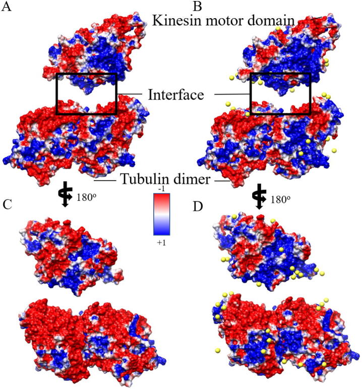
Electrostatic surface representation for kinesin dataset in front (A and B) and back side (C and D), in which A and C represent the electronic surface without explicit sodium ions (yellow balls) by the traditional method, and B and D represent the electronic surface with explicit sodium ions by the HIT. Images were rendered by Chimera with a color scale from −1.0 to 1.0 kT/e. (For interpretation of the references to color in this figure legend, the reader is referred to the web version of this article.)

Fig. 11.

Electrostatic surface representation of the interface between myosin motor domain and actin filament in two directions. A and C represent the electronic surface without explicit sodium ions (yellow balls) by the traditional method, and B and D represent the electronic surface with explicit sodium ions by the HIT. The images are rendered by Chimera with a color scale from −1.0 to 1.0 kT/e. (For interpretation of the references to color in this figure legend, the reader is referred to the web version of this article.)

Fig. 12.

Electrostatic surface representation for the interface between kinesin motor domain and tubulin dimer in two directions. A and C represent the electronic surface without explicit sodium ions (yellow balls) by the traditional method while B and D represent the electronic surface with explicit sodium ions by the HIT. The images are rendered by Chimera with a color scale from −1.0 to 1.0 kT/e. (For interpretation of the references to color in this figure legend, the reader is referred to the web version of this article.)

3.2.1. Compensation for net charge

As shown in Figs. 9 and 10, the comparison between the electrostatic surfaces calculated by the traditional method and by HIT shows that HIT significantly improved the electrostatic calculations. In Fig. 9A and C, the actin filament is highly negatively charged although some positive ions should be bound surrounding the actin filament. The lack of the bound positive ions causes unpredictable errors and bias in electrostatic calculations. By contrast, HIT (Fig. 9B and D) added the bound ions based on the ionic cloud distribution, neutralizing the actin filament. Similarly, as shown in Fig. 10, HIT improved the electrostatic calculation of the highly negatively charged tubulin dimer. Without HIT calculations, the electrostatic potential was calculated without any bound ions compensating for the highly charged system. For such highly charged systems, it is unrealistic to have no bound ions. We selected five positions (Fig. S6) to quantitatively compare the electrostatic potential calculations without and with HIT. These five points’ potential values were calculated by DelphiForce [48]. The results show that the average potential error was reduced from 0.93 to 0.53 kT/e in kinesin testing set by HIT (Fig. S6). Such bound ions added by HIT improve the electrostatic potential calculations and make it more realistic.

Fig. 11 illustrates the details on the interfaces of myosin-actin complex. The myosin binding interface is positive, and the actin filament binding interface is highly negative. Such electrostatic distributions generate the attractive forces between the myosin motor domain and the actin filament. With the traditional method, the interface of myosin is positive, as shown in blue regions in Fig. 11A and C. HIT added bound ions, which enlarged the positive area on the interface of myosin (Fig. 11B and D). Such bound ions may enhance the binding forces between the myosin and actin filament. The actin filament was highly negatively charged, and HIT added bound ions, shrinking the negative binding surfaces on the actin filament. In previous studies, the adjustment of the binding process is controlled by myosin binding protein and is widely accepted C [33]. It is thought to happen during the prepower stroke state [30], [49]. The shrunk negatively charged surface may be also related to the adjustment of the binding process, making the binding more specific.

Fig. 12 illustrates the details on the interfaces of the kinesin-tubulin dimer complex. In the traditional method (Fig. 12A and C), the interface of the kinesin motor domain is positively charged, and that of the tubulin dimer is negatively charged. The oppositely charged interfaces generate intensive binding forces. As with the effects on myosin, HIT enlarged the positive area on the kinesin interface by adding bound ions (Fig. 12B and D), strengthening the binding force on the interface. However, the additional bound ions shrank the positively charged area of the interface of the tubulin dimer, enhancing the specificity of the binding site.

3.2.2. The interactions between myosin motor domain and actin filament

The myosin motor domain and actin filament were separated by 20 Å for better visualization of electrostatic field lines (Fig. 13). The electrostatic figures were rendered by VMD. The density of the electrostatic field lines represents the strength of interactions between proteins. The actin filament includes G-actin and tropomyosin (TM). The interfaces between myosin motor domain and TM show intensely attractive interactions (Fig. 13 Left), but the interfaces between the myosin motor domain and G-actin yield much weaker interactions (Fig. 13 Right). In previous TM studies [50], the opinion about the movements of TM includes three states: open, close, and block states. They are thought to be regulated by Ca²⁺ activating troponin (Tn) to shift the position of TM. In some studies, myosin induces another movement of TM, which is about 10^° [35] or 23 Å [51], after myosin binding to actin filament. The interactions between myosin motor domain and TM provide evidence of myosin-regulated movement of TM [51]. By contrast, there are no distinct electrostatic interactions between myosin motor domain and G-actins (Fig. 13 Right), which are regarded as the main binding sites for myosin motor domain. Julian von der Ecken showed that the HLH motif of myosin enters the hydrophobic groove between actins to generate strong binding force [52]. Additionally, the main binding part of cardiomyopathy loop (CM-loop) is also primarily stabilized by hydrophobic interactions [52]. With support from the electrostatic studies, the electrostatic force does not dominate the interaction between myosin and G-actins.

Fig. 13.

Electrostatic field line for the interface of myosin motor domain with tropomyosin (Left enlarged view) and actin (Right enlarged view). Yellow balls represent explicit sodium ions added by the HIT. (For interpretation of the references to color in this figure legend, the reader is referred to the web version of this article.)

3.2.3. The interactions between the kinesin motor domain and the tubulin dimer

The kinesin motor domain and tubulin dimer were separated by 20 Å to better visualize the electrostatic field lines (Fig. 14). There were two intensely attractive interactions between cut7 kinesin motor domain and the tubulin dimer. One was on the interface of cut7/α-tubulin and the other was on the interface of cut7/β-tubulin. The binding strengths of cut7/α-tubulin and cut7/β-tubulin were similar. This is consistent with the distribution of charges on the interface of the kinesin motor domain and the tubulin dimer, as shown in Fig. 11B and D. Most kinesins interact with only β-tubulin [53], [54], but kinesin-5 (cut7) interacts with both α- and β-tubulin. This may imply the bidirectional characteristic of kinesin-5 (cut-7) [41].

Fig. 14.

Electrostatic field line for the interface of kinesin motor domain with α-tubulin (Left enlarged view) and kinesin motor domain with β-tubulin (Right enlarged view). Yellow balls represent explicit sodium ions added by the HIT. (For interpretation of the references to color in this figure legend, the reader is referred to the web version of this article.)

4. Conclusions

Ions are important to balance the net charges of highly charged biomolecules, and bound ions are crucial for the functions of highly charged biomolecules, such as DNAs, RNAs, and other biomolecules. In computational simulations, treating the ions properly is challenging essential. In this work, we developed a novel method, the hybridizing ions treatment (HIT), which hybridizes the implicit solvent method and explicit method to realistically calculate the electrostatic potential of highly charged biomolecules.

The implementation of HIT on two multiprotein complexes shows that this method improved the electrostatic calculations significantly. It predicted the positions of bound ions and then utilized the bound ions to neutralize the biomolecules, thus providing more realistic electrostatic calculations. The electrostatic interaction between the actin filament and the myosin motor domain proved that the electrostatic interactions between the myosin motor domain and the TM was stronger than that between the myosin motor domain and G-actin, revealing the mechanism of the myosin-regulated motion of the TM, which has been observed experimentally [35], [51]. The interaction between cut7 kinesin motor domain and the tubulin dimer was calculated; it demonstrated that the binding strengths of cut7/α-tubulin and cut7/β-tubulin were similar. Such similar electrostatic binding interactions may be a reason of the bidirectional motility feature for cut7 [41].

Besides the two applications in this work, application of HIT would be useful in many other fields related to highly charged biomolecules, including DNAs, RNAs, molecular motors, and other biomolecules. In this work, we used Na⁺ as a test case. The performance of HIT is independent of ion types because HIT utilizes information about ion distribution from MD simulations to analyze which ions are bound. Current MD algorithms treat different types of ions very reliably; thus, HIT can be expected to handle other types of ions as well as it did Na⁺. However, a limitation of HIT is that it can be applied to only biomolecules that do not have large conformational changes. For structures with such changes, more comprehensive algorithms would be necessary to predict bound ions. In our test sets, protein conformations changed only a little. Our future work will focus on the problem of biomolecules that undergo large conformational changes. The supplementary material and the data in this work (including training set and results) are available online. The HIT package is available at http://compbio.utep.edu/static/downloads/download_hit.zip.

Declaration of Competing Interest

The authors declare that they have no known competing financial interests or personal relationships that could have appeared to influence the work reported in this paper.

Appendix A. Supplementary data

The following are the Supplementary data to this article:

References

- 1.Ganguly D., Otieno S., Waddell B., Iconaru L., Kriwacki R.W., Chen J. Electrostatically accelerated coupled binding and folding of intrinsically disordered proteins. J Mol Biol. 2012;422:674–684. doi: 10.1016/j.jmb.2012.06.019. [DOI] [PMC free article] [PubMed] [Google Scholar]
- 2.Stigter D., Alonso D.O., Dill K.A. Protein stability: electrostatics and compact denatured states. Proc Natl Acad Sci. 1991;88:4176–4180. doi: 10.1073/pnas.88.10.4176. [DOI] [PMC free article] [PubMed] [Google Scholar]
- 3.Strickler S.S., Gribenko A.V., Gribenko A.V., Keiffer T.R., Tomlinson J., Reihle T. Protein stability and surface electrostatics: a charged relationship. Biochemistry. 2006;45:2761–2766. doi: 10.1021/bi0600143. [DOI] [PubMed] [Google Scholar]
- 4.Zondlo N.J. Aromatic–proline interactions: electronically tunable CH/π interactions. Acc Chem Res. 2013;46:1039–1049. doi: 10.1021/ar300087y. [DOI] [PMC free article] [PubMed] [Google Scholar]
- 5.Li L., Jia Z., Peng Y., Godar S., Getov I., Teng S. Forces and Disease: Electrostatic force differences caused by mutations in kinesin motor domains can distinguish between disease-causing and non-disease-causing mutations. Sci Rep. 2017;7:1–12. doi: 10.1038/s41598-017-08419-7. [DOI] [PMC free article] [PubMed] [Google Scholar]
- 6.Li L., Wang L., Alexov E. On the energy components governing molecular recognition in the framework of continuum approaches. Front Mol Biosci. 2015;2:5. doi: 10.3389/fmolb.2015.00005. [DOI] [PMC free article] [PubMed] [Google Scholar]
- 7.Richardson J.S., Richardson D.C. Helix lap-joints as ion-binding sites: DNA-binding motifs and Ca-binding “EF hands” are related by charge and sequence reversal. Proteins Struct Funct Bioinforma. 1988;4:229–239. doi: 10.1002/prot.340040402. [DOI] [PubMed] [Google Scholar]
- 8.Akhtar A., Zink D., Becker P.B. Chromodomains are protein–RNA interaction modules. Nature. 2000;407:405–409. doi: 10.1038/35030169. [DOI] [PubMed] [Google Scholar]
- 9.Nicholls A., Honig B. A rapid finite difference algorithm, utilizing successive over-relaxation to solve the Poisson-Boltzmann equation. J Comput Chem. 1991;12:435–445. [Google Scholar]
- 10.Jayaram B., Sprous D., Beveridge D.L. Solvation free energy of biomacromolecules: Parameters for a modified generalized Born model consistent with the AMBER force field. J Phys Chem B. 1998;102:9571–9576. [Google Scholar]
- 11.Klapper I., Hagstrom R., Fine R., Sharp K., Honig B. Focusing of electric fields in the active site of Cu-Zn superoxide dismutase: effects of ionic strength and amino-acid modification. Proteins Struct Funct Bioinforma. 1986;1:47–59. doi: 10.1002/prot.340010109. [DOI] [PubMed] [Google Scholar]
- 12.Jia Z., Li L., Chakravorty A., Alexov E. Treating ion distribution with G aussian-based smooth dielectric function in DelPhi. J Comput Chem. 2017;38:1974–1979. doi: 10.1002/jcc.24831. [DOI] [PMC free article] [PubMed] [Google Scholar]
- 13.Florová P., Sklenovský P., Banáš P., Otyepka M. Explicit water models affect the specific solvation and dynamics of unfolded peptides while the conformational behavior and flexibility of folded peptides remain intact. J Chem Theory Comput. 2010;6:3569–3579. doi: 10.1021/ct1003687. [DOI] [PubMed] [Google Scholar]
- 14.Li L., Li C., Sarkar S., Zhang J., Witham S., Zhang Z. DelPhi: a comprehensive suite for DelPhi software and associated resources. BMC Biophys. 2012;5:9. doi: 10.1186/2046-1682-5-9. [DOI] [PMC free article] [PubMed] [Google Scholar]
- 15.Li L., Li C., Zhang Z., Alexov E. %J J of chemical theory, computation. On the dielectric “constant” of proteins: smooth dielectric function for macromolecular modeling and its implementation in DelPhi. J Chem Theory Comput. 2013;9:2126–2136. doi: 10.1021/ct400065j. [DOI] [PMC free article] [PubMed] [Google Scholar]
- 16.Wei Y.-L., Yang W.-X. Kinesin-14 motor protein KIFC1 participates in DNA synthesis and chromatin maintenance. Cell Death Dis. 2019;10:1–14. doi: 10.1038/s41419-019-1619-9. [DOI] [PMC free article] [PubMed] [Google Scholar]
- 17.Li L., Alper J., Alexov E. Cytoplasmic dynein binding, run length, and velocity are guided by long-range electrostatic interactions. Sci Rep. 2016;6:31523. doi: 10.1038/srep31523. [DOI] [PMC free article] [PubMed] [Google Scholar]
- 18.Li M., Zheng W. All-atom molecular dynamics simulations of actin-myosin interactions: a comparative study of cardiac α myosin, β myosin, and fast skeletal muscle myosin. Biochemistry. 2013;52:8393–8405. doi: 10.1021/bi4006896. [DOI] [PubMed] [Google Scholar]
- 19.Baker N.A., Sept D., Joseph S., Holst M.J., McCammon J.A. %J P of the NA of S. Electrostatics of nanosystems: application to microtubules and the ribosome. Proc Natl Acad Sci. 2001;98:10037–10041. doi: 10.1073/pnas.181342398. [DOI] [PMC free article] [PubMed] [Google Scholar]
- 20.De Graff A.M.R., Hazoglou M.J., Dill K.A. Highly charged proteins: the Achilles’ heel of aging proteomes. Structure. 2016;24:329–336. doi: 10.1016/j.str.2015.11.006. [DOI] [PubMed] [Google Scholar]
- 21.Lee K.K., Fitch C.A., Lecomte J.T.J., García-Moreno E.B. Electrostatic effects in highly charged proteins: salt sensitivity of p K a values of histidines in staphylococcal nuclease. Biochemistry. 2002;41:5656–5667. doi: 10.1021/bi0119417. [DOI] [PubMed] [Google Scholar]
- 22.Dayton W.R., Reville W.J., Goll D.E., Stromer M.H. %J B. A calcium (2+) ion-activated protease possibly involved in myofibrillar protein turnover. Partial characterization of the purified enzyme. Biochemistry. 1976;15:2159–2167. doi: 10.1021/bi00655a020. [DOI] [PubMed] [Google Scholar]
- 23.Yamada Y., Namba K., Fujii T. %J N communications. Cardiac muscle thin filament structures reveal calcium regulatory mechanism. Nat Commun. 2020;11:1–9. doi: 10.1038/s41467-019-14008-1. [DOI] [PMC free article] [PubMed] [Google Scholar]
- 24.Zhou S., Cheng L.-T., Dzubiella J., Li B., Mccammon J.A. Variational implicit solvation with Poisson−Boltzmann theory. ACS Publ. 2014;10:1454–1467. doi: 10.1021/ct401058w. [DOI] [PMC free article] [PubMed] [Google Scholar]
- 25.Zhou S., Cheng L.T., Sun H., Che J., Dzubiella J., Li B. LS-VISM: a software package for analysis of biomolecular solvation. J Comput Chem. 2015;36:1047–1059. doi: 10.1002/jcc.23890. [DOI] [PMC free article] [PubMed] [Google Scholar]
- 26.Zhou S, Weiß R, … LC-P of the, 2019 undefined. Variational implicit-solvent predictions of the dry–wet transition pathways for ligand–receptor binding and unbinding kinetics. Natl Acad Sci n.d. [DOI] [PMC free article] [PubMed]
- 27.Shashikala HBM, Chakravorty A, Pandey S, Alexov E. BION-2: Predicting positions of non-specifically bound ions on protein surface by a Gaussian-based treatment of electrostatic environment. 2020. [DOI] [PMC free article] [PubMed]
- 28.Phillips J.C., Braun R., Wang W., Gumbart J., Tajkhorshid E., Villa E. Scalable molecular dynamics with NAMD. J Comput Chem. 2005;26:1781–1802. doi: 10.1002/jcc.20289. [DOI] [PMC free article] [PubMed] [Google Scholar]
- 29.Dolinsky T.J., Nielsen J.E., McCammon J.A., Baker N.A. PDB2PQR: an automated pipeline for the setup of Poisson-Boltzmann electrostatics calculations. Nucleic Acids Res. 2004;32:W665–W667. doi: 10.1093/nar/gkh381. [DOI] [PMC free article] [PubMed] [Google Scholar]
- 30.Houdusse A., Sweeney H.L. How myosin generates force on actin filaments. Trends Biochem Sci. 2016;41:989–997. doi: 10.1016/j.tibs.2016.09.006. [DOI] [PMC free article] [PubMed] [Google Scholar]
- 31.Geisterfer-Lowrance A.A.T., Kass S., Tanigawa G., Vosberg H.-P., McKenna W., Seidman C.E. A molecular basis for familial hypertrophic cardiomyopathy: a β cardiac myosin heavy chain gene missense mutation. Cell. 1990;62:999–1006. doi: 10.1016/0092-8674(90)90274-i. [DOI] [PubMed] [Google Scholar]
- 32.Burghardt T.P., Sikkink L.A. Regulatory light chain mutants linked to heart disease modify the cardiac myosin lever arm. Biochemistry. 2013;52:1249–1259. doi: 10.1021/bi301500d. [DOI] [PMC free article] [PubMed] [Google Scholar]
- 33.Inchingolo A.V., Previs S.B., Previs M.J., Warshaw D.M., Kad N.M. Revealing the mechanism of how cardiac myosin-binding protein C N-terminal fragments sensitize thin filaments for myosin binding. Proc Natl Acad Sci. 2019;116:6828–6835. doi: 10.1073/pnas.1816480116. [DOI] [PMC free article] [PubMed] [Google Scholar]
- 34.Robert-Paganin J., Auguin D., Houdusse A. Hypertrophic cardiomyopathy disease results from disparate impairments of cardiac myosin function and auto-inhibition. Nat Commun. 2018;9:1–13. doi: 10.1038/s41467-018-06191-4. [DOI] [PMC free article] [PubMed] [Google Scholar]
- 35.Risi C., Eisner J., Belknap B., Heeley D.H., White H.D., Schröder G.F. Ca2+-induced movement of tropomyosin on native cardiac thin filaments revealed by cryoelectron microscopy. Proc Natl Acad Sci. 2017;114:6782–6787. doi: 10.1073/pnas.1700868114. [DOI] [PMC free article] [PubMed] [Google Scholar]
- 36.AL-Khayat H.A. Three-dimensional structure of the human myosin thick filament: clinical implications. Glob Cardiol Sci Pract. 2013;2013:36. doi: 10.5339/gcsp.2013.36. [DOI] [PMC free article] [PubMed] [Google Scholar]
- 37.Luther P.K., Winkler H., Taylor K., Zoghbi M.E., Craig R., Padrón R. Direct visualization of myosin-binding protein C bridging myosin and actin filaments in intact muscle. Proc Natl Acad Sci. 2011;108:11423–11428. doi: 10.1073/pnas.1103216108. [DOI] [PMC free article] [PubMed] [Google Scholar]
- 38.Li L., Alper J., Alexov E. Multiscale method for modeling binding phenomena involving large objects: application to kinesin motor domains motion along microtubules. 2016;6:23249. doi: 10.1038/srep23249. [DOI] [PMC free article] [PubMed] [Google Scholar]
- 39.Kapitein L.C., Peterman E.J.G., Kwok B.H., Kim J.H., Kapoor T.M., Schmidt C.F. The bipolar mitotic kinesin Eg5 moves on both microtubules that it crosslinks. Nature. 2005;435:114–118. doi: 10.1038/nature03503. [DOI] [PubMed] [Google Scholar]
- 40.Huszar D., Theoclitou M.-E., Skolnik J., Herbst R. %J C, Reviews M. Kinesin motor proteins as targets for cancer therapy. Cancer Metastasis Rev. 2009;28:197–208. doi: 10.1007/s10555-009-9185-8. [DOI] [PubMed] [Google Scholar]
- 41.von Loeffelholz O., Peña A., Drummond D.R., Cross R., Moores C.A. Cryo-EM structure (4.5-Å) of yeast kinesin-5–microtubule complex reveals a distinct binding footprint and mechanism of drug resistance. J Mol Biol. 2019;431:864–872. doi: 10.1016/j.jmb.2019.01.011. [DOI] [PMC free article] [PubMed] [Google Scholar]
- 42.Humphrey W., Dalke A., Schulten K. VMD: visual molecular dynamics. J Mol Graph. 1996;14:33–38. doi: 10.1016/0263-7855(96)00018-5. [DOI] [PubMed] [Google Scholar]
- 43.Vanommeslaeghe K., Hatcher E., Acharya C., Kundu S., Zhong S., Shim J. CHARMM general force field: a force field for drug-like molecules compatible with the CHARMM all-atom additive biological force fields. J Comput Chem. 2010;31:671–690. doi: 10.1002/jcc.21367. [DOI] [PMC free article] [PubMed] [Google Scholar]
- 44.Li C., Li L., Zhang J., Alexov E. Highly efficient and exact method for parallelization of grid-based algorithms and its implementation in DelPhi. J Comput Chem. 2012;33:1960–1966. doi: 10.1002/jcc.23033. [DOI] [PMC free article] [PubMed] [Google Scholar]
- 45.Li C., Petukh M., Li L., Alexov E. Continuous development of schemes for parallel computing of the electrostatics in biological systems: implementation in DelPhi. J Comput Chem. 2013;34:1949–1960. doi: 10.1002/jcc.23340. [DOI] [PMC free article] [PubMed] [Google Scholar]
- 46.Li C., Jia Z., Chakravorty A., Pahari S., Peng Y., Basu S. DelPhi suite: new developments and review of functionalities. J Comput Chem. 2019;40:2502–2508. doi: 10.1002/jcc.26006. [DOI] [PMC free article] [PubMed] [Google Scholar]
- 47.Pettersen E.F., Goddard T.D., Huang C.C., Couch G.S., Greenblatt D.M., Meng E.C. UCSF Chimera - a visualization system for exploratory research and analysis. J Comput Chem. 2004 doi: 10.1002/jcc.20084. [DOI] [PubMed] [Google Scholar]
- 48.Li L., Chakravorty A., Alexov E. DelPhiForce, a tool for electrostatic force calculations: applications to macromolecular binding. J Comput Chem. 2017;38:584–593. doi: 10.1002/jcc.24715. [DOI] [PMC free article] [PubMed] [Google Scholar]
- 49.Llinas P., Isabet T., Song L., Ropars V., Zong B., Benisty H. How actin initiates the motor activity of Myosin. Dev Cell. 2015;33:401–412. doi: 10.1016/j.devcel.2015.03.025. [DOI] [PMC free article] [PubMed] [Google Scholar]
- 50.Yamada Y., Namba K., Fujii T. Cardiac muscle thin filament structures reveal calcium regulatory mechanism. Nat Commun. 2020;11:1–9. doi: 10.1038/s41467-019-14008-1. [DOI] [PMC free article] [PubMed] [Google Scholar]
- 51.Behrmann E., Müller M., Penczek P.A., Mannherz H.G., Manstein D.J., Raunser S. Structure of the rigor actin-tropomyosin-myosin complex. Cell. 2012;150:327–338. doi: 10.1016/j.cell.2012.05.037. [DOI] [PMC free article] [PubMed] [Google Scholar]
- 52.von der Ecken J., Heissler S.M., Pathan-Chhatbar S., Manstein D.J., Raunser S. Cryo-EM structure of a human cytoplasmic actomyosin complex at near-atomic resolution. Nature. 2016;534:724–728. doi: 10.1038/nature18295. [DOI] [PubMed] [Google Scholar]
- 53.Hunter B., Allingham J.S. These motors were made for walking. Protein Sci. 2020 doi: 10.1002/pro.3895. [DOI] [PMC free article] [PubMed] [Google Scholar]
- 54.Woehlke G., Ruby A.K., Hart C.L., Ly B., Hom-Booher N., Vale R.D. Microtubule interaction site of the kinesin motor. Cell. 1997;90:207–216. doi: 10.1016/s0092-8674(00)80329-3. [DOI] [PubMed] [Google Scholar]
Associated Data
This section collects any data citations, data availability statements, or supplementary materials included in this article.