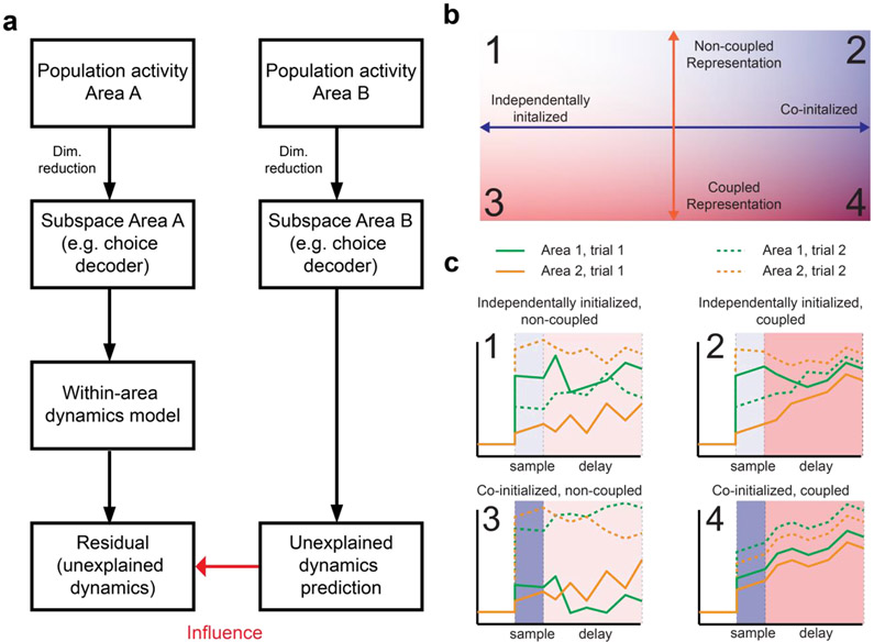
Figure 3. A schematic of predictive model analysis for multi-regional interactions and interpretations in terms of co-initialization and dynamic coupling.
a. Flow chart for predictive model analysis at the population level. To infer influence of Area B on Area A, we measure how much of future activity in Area A that cannot be predicted from its own past activity, can be predicted from past activity in Area B. More specifically, we first model the within-area dynamics of Area A to predict its future activity. The residual of this within-area prediction is then predicted from Area B, the performance of which defines a measure of influence from Area B to A. To avoid potential overfitting, one can first apply dimensionality reduction to the raw population activity in each area and focus on task-relevant activity components (such as the projection onto CD).
b. Correlated activity across brain areas could be described through co-initialization of two brain areas (Quadrant 2), dynamic coupling between them (Quadrant 3), or a combination of both (Quadrant 4).
c. Schematics of single-trial trajectories of activities in the two areas illustrating each condition. Population activity in each area is assumed to be projected onto a low-dimensional subspace of interest, such as CD. Green, area 1; orange, area 2. Solid lines, trial 1; dashed lines, trial 2. Top left, independently initialized, non-coupled (Quadrant 1). The initial states of the two areas during the sample period are uncorrelated, and they evolve independently from each other. Top right, independently initialized, coupled (Quadrant 2). While the initial states of the two areas are uncorrelated, their interactions tend to make their states more correlated over time. Bottom left, co-initialized, non-coupled (Quadrant 3). While the initial states of the two areas are correlated, their subsequent states gradually become more independent. Bottom right, co-initialized, coupled (Quadrant 4). The states of the two areas remain highly correlated across both the sample and delay period.

