Figure 2.

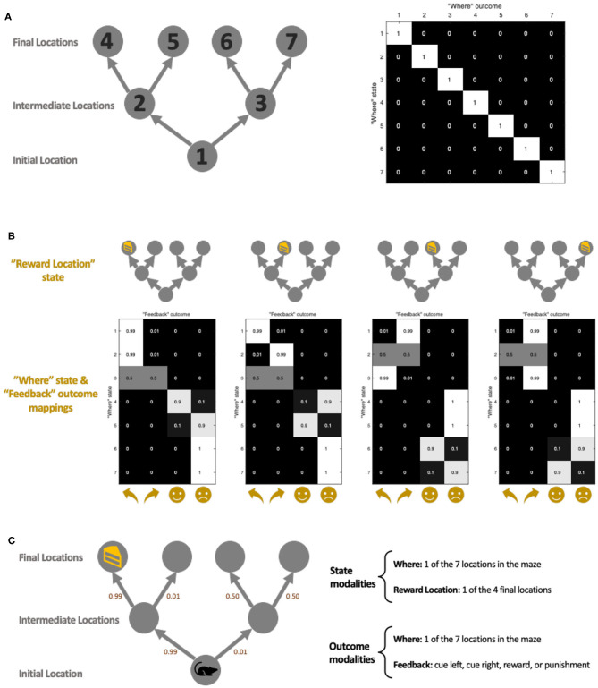
Simulation maze set-up. (A) The maze location set-up. There are a total of 7 locations in the maze, each with their corresponding indexes (left diagram). The state-outcome mapping (A matrix) between “Where” (i.e., agent's current location) state and outcome is an identity matrix (right figure), meaning they always correspond exactly. The maze consists of three stages: initial, intermediate, and final. The state-state transition matrix (B matrix) ensures that an agent can only move forward in the maze, following the direction of the arrow. (B) The state-outcome transition probability between the “Where” state and “Feedback” outcome (as encoded by the A matrix). Depending on the location of the reward, the agent receives different feedbacks which include a directional cue (cue left or cue right) in the initial and intermediate locations, and a reward or punishment at the final locations. The index of the y-axis corresponds with the location index in (A). Here we have depicted unambiguous cues, where the agent is 99% sure it sees the cue pointed in the correct (i.e., toward the reward location) cue. (C) An example maze set-up with a reward at the left-most final location. The agent starts in the initial location, and the agent's model-based brain contains representations of where it is in the maze, as well as where it thinks the reward is. The agent is able to make geographical observations to see where it is in the maze (A), as well as receive a “feedback” outcome which gives it a cue to go a certain location, or to give it reward/punishment (B). The small numbers beside each arrow illustrate the ambiguity of the cues. As an example, we have illustrated the left-most scenario of (B).