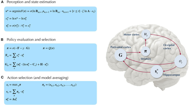
Figure 5.

Belief-updating under active inference. Overview of the update equations for posterior beliefs under active inference. (A) Shows the optimal solution for posterior beliefs about hidden states s^* that minimizes the variational free energy of observations. In practice the variational posterior over states is computed as a marginal message passing routine (Parr et al., 2019), where prediction errors ${\epsilon }_{\tau }^{\pi }$ minimized over time until some criterion of convergence is reached (ε ≈ 0). The prediction errors measure the difference between the current log posterior over states $ln{\text{s}}_{\tau }^{\pi }$ and the optimal solution ln s^*. Solving via error-minimization lends the scheme a degree of biological plausibility and is consistent with process theories of neural function like predictive coding (Bastos et al., 2012; Bogacz, 2017). An alternative scheme would be equating the marginal posterior over hidden states (for a given factor and/or timestep) to the optimal solution ${\text{s}}_{\pi ,\tau }^{*}$—this is achieved by solving for s^* when free energy is at its minimum (for a particular marginal), i.e., $\frac{\partial F}{\partial {\text{s}}_{\pi ,\tau }}=0$. This corresponds to a fixed-point minimization scheme (also known as coordinate-ascent iteration), where each conditional marginal is iteratively fixed to its free-energy minimum, while holding the remaining marginals constant (Blei et al., 2017). (B) Shows how posterior beliefs about policies are a function of the free energy of states expected under policies F and the expected free energy of policies G. F is a function of state prediction errors and expected states, and G is the expected free energy of observations under policies, shown here decomposed into the KL divergence between expected and preferred observations or risk (${\text{o}}_{\tau }^{\pi }·(ln{\text{o}}_{\tau }^{\pi }-{\text{C}}_{\tau })$) and the expected entropy or ambiguity ($\text{H}·{\text{s}}_{\tau }^{\pi }$). A precision parameter γ scales the expected free energy and serves as an inverse temperature parameter for a softmax normalization σ of policies. See the text (Section 4.1.1) for more clarification on the free energy of policies F. (C) Shows how actions are sampled from the posterior over policies, and the posterior over states is updated via a Bayesian model average, where expected states are averaged under beliefs about policies. Finally, expected observations are computed by passing expected states through the likelihood of the generative model. The right side shows a plausible correspondence between several key variables in an MDP generative model and known neuroanatomy. For simplicity, a hierarchical generative model is not shown here, but one can easily imagine a hierarchy of state inference that characterizes the recurrent message passing between lower-level occipital areas (e.g., primary visual cortex) through higher level visual cortical areas, and terminating in “high-level,” prospective and policy-conditioned state estimation in areas like the hippocampus. We note that it is an open empirical question, whether various computations required for active inference can be localized to different functional brain areas. This figure suggests a simple scheme that attributes different computations to segregated brain areas, based on their known function and neuroanatomy (e.g., computing the expected free energy of actions (G), speculated to occur in frontal areas).