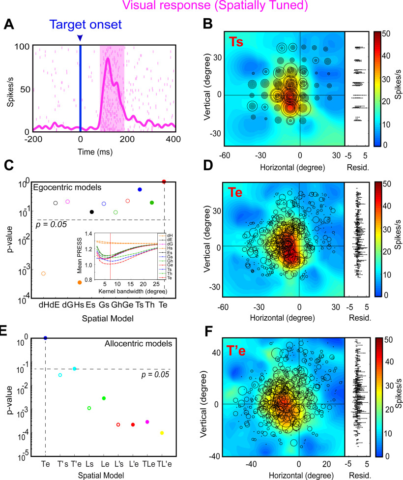
Figure 5.

An example of response field analysis of a visual neuron. A, Raster/spike density plot (with top 10% responses) of the visual neuron aligned to the onset of target (blue arrow); the shaded pink region corresponds to the sampling window (80–180 ms) for response field analysis. B, Representation of neural activity for Ts: target in space (screen). The circle corresponds to the magnitude of the response and heat map represents the non-parametric fit to these data (red blob depicts the hot-spot of the neuronal response field). The corresponding residuals are displayed to the right. To independently compute the residual for a trial, its activity was subtracted from the point corresponding to the fit computed on the rest of the trials. The residuals are one-dimensional for every data point from the fit projected onto the vertical axis for illustrative purposes. C, The p value statistics and comparison between Te (p = 10° = 1; the best-fit spatial model that yielded lowest residuals) and other tested models (Brown–Forsythe test). Inset shows the mean residuals from the PRESS-statistics for all spatial models at different kernel bandwidths (2–25°). The red vertical line depicts the lowest mean PRESS for Te (target in eye coordinates) with a kernel bandwidth of 7. D, Representation of the neural activity in Te (target relative to eye), the best coordinate. E, The p value statistics and the comparison of the best egocentric model, Te, with other allocentric spatial models. Te is still the best-fit model. F, Representation of the neural activity in T’e, i.e., shifted target relative eye; 0, 0 represents the center of the coordinate system that led to the lowest residuals (best fit).