Abstract
This study provides a detailed exposition of in-hospital community-acquired methicillin-resistant S. aureus (CA-MRSA) which is a new strain of MRSA, and hospital-acquired methicillin-resistant S. aureus (HA-MRSA) employing Caputo fractional operator. These two strains of MRSA, referred to as staph, have been a serious problem in hospitals and it is known that they give rise to more deaths per year than AIDS. Hence, the transmission dynamics determining whether the CA-MRSA overtakes HA-MRSA is analyzed by means of a non-local fractional derivative. We show the existence and uniqueness of the solutions of the fractional staph infection model through fixed-point theorems. Moreover, stability analysis and iterative solutions are furnished by the recursive procedure. We make use of the parameter values obtained from the Beth Israel Deaconess Medical Center. Analysis of the model under investigation shows that the disease-free equilibrium existing for all parameters is globally asymptotically stable when both and are less than one. We also carry out the sensitivity analysis to identify the most sensitive parameters for controlling the spread of the infection. Additionally, the solution for the above-mentioned model is obtained by the Laplace-Adomian decomposition method and various simulations are performed by using convenient fractional-order .
Keywords: Fractional operators, Caputo derivative, Staph infection, Laplace-Adomian decomposition method, Staphylococcus aureus
Introduction
Many compartmental models like SIS, SIR, SIRS, SEIRS, MSEIR, MSEIRS have been introduced since 1927 in order to analyze the infectious diseases in detail by means of mathematical tools. When analyzed such models, it is supposed that the population is in a homogeneous structure, people react the same to infectious diseases and transform from one situation to another collectively. We should emphasize that this significant assumption is essential for formulating a complex system. Infectious diseases that cannot be fully defined have taken a crucial role in shaping world history while reducing the world population. For instance, in the second century AD, Antonine Plague gave rise to a sharp decline in the population and economic trouble in the Roman Empire and so this disease that caused the disruption of order led to the collapse of the Roman Empire. On the other hand, the Han empire also collapsed owing to similar reasons in the third century AD. The plague epidemic, which started in the Eastern Roman Empire in 541, affected the Mediterranean region adversely until 750 and caused an estimated 20-30 percent decrease in the population. With infectious diseases such as smallpox, measles, and diphtheria, 90 percent of the indigenous people died, and their population, which was 30 million in Mexico, decreased to 3 million between 1519–1530. Moreover, the plague called Black Death that ended up with great destruction between 1347 and 1351 destroyed about a third of the European population, which was 70 million in the 1340s and it repeated regularly more than 300 years in many parts of Europe. Also in the nineteenth century, cholera killed millions of people, and in 1918-1919 influenza killed more than 20 million people in the United States [1]. Between June 1918 and December 1920, Spanish Flu, the deadliest pandemic, caused the death of at least 50 million people, which constituted about 3 percent of the world population, and 500 million people were affected by this virus in almost every region of the world [2].
The increase in the effectiveness of sanitation programs, antibiotics, and vaccination programs in the 1960s led to the idea that infectious diseases will be overcome. Furthermore, infectious diseases adapt and develop in new environments and also new ecosystems, global warming, rise in international travel, changes in the economic structure allow novel infectious diseases to emerge easier. Resistance to antibiotics utilized in gonorrhea, tuberculosis, and pneumonia has developed and some diseases like dengue fever, yellow fever, malaria have become widespread especially in regions where climate change is experienced [3, 4]. In the last 40 years, various new infectious diseases such as Lyme (1975), legionary (1976), toxic shock syndrome (1978), hepatitis C (1989), hepatitis E (1990), hantavirus (1993), hepatitis G (1995), Nipah (1998), SARS (2003) have been diagnosed [5]. The Human Immunodeficiency Virus (HIV), the etiological agent (infectious substances) for Acquired Immune Deficiency Syndrome (AIDS), was first diagnosed in 1981 and surrounded the world. According to 2009 data, AIDS was a crucial infectious disease that caused about 25 million deaths and 33 million people had to live together with this dangerous disease and fight to death [6].
Numerous deaths due to plague, smallpox, cholera, and influenza outbreaks have led to the creation of various models for the monitoring and prevention of the spread of infectious diseases since the 17th century. Initially, it was aimed at monitoring only the simple data collection and the increase and decrease in the number of deaths, but today, the models are set using all the possibilities of information and communication technologies. In this context, system dynamics and agent-based simulation models, geographic information systems, spatial data mining, complex networks, heuristic methods, and dynamic system approaches play an important role. The basics of all these methods are based on mathematical models that seek solutions with differential equations laid in the 1920s. The first mathematical model related to infectious diseases belongs to Daniel Bernoulli published in 1766. In Bernoulli’s study, variolation discussions, a vaccination method developed for smallpox, are tackled by means of a mathematical model [7]. In 1906, Hamer designed and analyzed a discrete-time model to examine the recurrence of measles outbreaks. The model is important because it is the first model that assumes that the number of new cases that occur per unit time depends on the number of susceptible and disease-carrying individuals. After these studies, A. G. McKendrick and W. O. Kermack made the biggest contribution, which was shown as the first example in the prediction of the spread of infectious diseases by means of mathematical models and published in 1927 [8].
As an example of the SIS model, let us make mention of the spread of staph infection in hospitals. Methicillin-resistant Staphylococcus aureus (MRSA) is a bacterium that can cause serious infections in humans and is often referred to as staph. In fact, this bacterium is resistant to the typically used antibiotic methicillin. In hospitals, patients with compromised immune systems or elderly patients can easily catch the MRSA bacterium and get bloodstream infectious. MRSA, traditionally a crucial problem in hospitals, accounts for the significant part of hospital fatalities and brings about more deaths than AIDS each year [9]. Recently, a different genetic type of MRSA has been identified and it has been found that this novel strain CA-MRSA can also infect healthy and young individuals while traditional strain HA-MRSA has occasionally. In some studies, it is asserted that CA-MRSA may surpass HA-MRSA and so deaths may increase yearly owing to the severity of the problem handled. Therefore, a compartmental mathematical model has been developed to determine whether the CA-MRSA overtakes HA-MRSA. For more details on the above-mentioned model, we refer the reader to [9].
Fractional calculus, a venerable branch of mathematical analysis, examines the possibilities of the order of the derivative and integral operator, which is generally denoted by D and I, to be real or complex number. Although the idea of fractional derivative was first introduced when L’Hopital asked a question about fractional derivative to Leibniz in 1695, the definition of fractional derivative was not presented by Leibniz at that time. Hence, the fractional derivative definition has been put forward by subsequent scientists and today has many applications in biology, physics, chemistry, engineering, and so on. The topic of fractional calculus has attracted great attention from several authors due to applicability to various real-world problems and has the potential to achieve better results than the classical derivative [10, 11]. The most common way of explaining fractional operators is to present the Riemann-Liouville (RL) integral and derivative of an arbitrary complex analytic function. These substantial definitions are given as follows
| 1 |
| 2 |
respectively. However, the definition of RL is not sufficient to fully explain fractional calculus because it has some shortcomings in practice related to initial conditions. So, various fractional derivatives with a wide variety of properties have been defined to compensate for these shortcomings. It should be emphasized that in fractional calculus, unlike classical analysis, there are dozens of differintegral definitions instead of a specific definition. This active and popular field of research has great importance for the modeling of certain biological, physical, etc processes. For more information on fractional operators, see [12–23] and the references given there. On the other hand, Caputo fractional derivative obtained by modifying the Riemann-Liouville definition is of paramount significance because of the applicability to various problems in daily life [24]. So, we present the definition of Caputo fractional operator as below:
| 3 |
where and . From the applications point of view, this useful fractional derivative has been widely interpreted in connection with different areas such as finance, diffusion, control engineering, optics, non-Markovian physical processes, etc. One of the best ways to comprehend the fractional calculus is to consider the tautochrone problem in which non-integer order is needed to get the desired results. It can be predicted that in the future, a definition covering all definitions of fractional operators available in the literature may be introduced. To learn more about the content of this study, we refer the readers to [25–43].
In hospitals, the infection of MRSA, a gram-positive bacterium, has traditionally been a crucial problem causing many deaths each year. Hospital-acquired MRSA strain (HA-MRSA) is usually seen in elderly people or patients with a weak immune system while community-acquired MRSA strain can also infect young and healthy individuals. Thus in order to critically enunciate the actual characteristics of the situation, an expansive study needs to be carried out. It can be noted that, in the recent past, multifarious scientists have shown that the fractional calculus can more precisely explain natural phenomena than the integer calculus. In light of these facts, fractional calculus has become increasingly important and common in modeling realistic cases, particularly those with memory effects. We get inspired to investigate and evaluate the fractional variant of the governing model with an effective fractional operator called Caputo fractional derivative. To the best of our knowledge, this is the first time a fractional operator has been employed for the analysis and investigation of the underlying model. Consequently, several properties of the model such as existence and uniqueness of the solution, positivity, stability analysis, sensitivity analysis, basic reproduction number have been analyzed. Furthermore, by means of an effective method called Laplace-Adomian decomposition method (LADM), simulation and comparative analysis are carried out on the basis of the model being considered and the values of parameters to determine the efficiency and effectiveness of the current fractional variant of the model in the Caputo sense.
The remainder of this study is as follows: In Sect 2, model description and necessary prerequisites are given in both classical and fractional manner. We show the existence and uniqueness of solutions related to the Caputo fractional derivative and some other crucial theoretical information such as stability analysis, sensitivity analysis, and so on are furnished in Sect. 3. Moreover, we present the solution for the MRSA model using the method of LADM related to Caputo’s definition and plot various graphs to get comparative results in Sect. 4. Finally, we give some important concluding remarks in Sect. 5.
Model description and prerequisites
In this segment, we present the methicillin-resistant Staphylococcus aereus (MRSA) model with two strains, CA-MRSA and HA-MRSA, by making use of standard works on the current model in [9, 23, 25]. Hence, the population exposed to an infectious disease in the model is divided into three groups:
patients colonized with HA-MRSA,
patients colonized with CA-MRSA,
susceptible patients who are not colonized with HA-MRSA or CA-MRSA.
The parameters of the model we studied are given as follows:
the total number of the individuals who are the patients in the hospital,
the daily entrance rate of patients to the hospital,
the daily exit rate of patients who are colonized with CA-MRSA through death or discharge,
the daily exit rate of patients who are colonized with HA-MRSA through death or discharge,
the daily exit rate of susceptible patients through death or discharge,
the daily transfer rate of CA-MRSA among patients,
the daily transfer rate of HA-MRSA among patients,
the daily rate of undergoing decolonization measures of patients who are colonized with CA-MRSA,
the daily rate of undergoing decolonization measures of patients who are colonized with HA-MRSA,
Susceptible patients denoted by S(t) can become contaminated when visited by the colonized healthcare team or as a result of failure to pay attention to hand hygiene, the healthcare team can become colonized by coming into contact with infected patients. The susceptible patient is the person who does not have enough immunity to prevent the infection that will occur with this factor when it is exposed to a certain pathogen. Also, C(t) and S(t) are infectious individuals who carry the disease and can transmit it to susceptible individuals. Although some people have a natural immunity to certain infectious diseases, individuals in this situation can be neglected in modeling as they will constitute a very small proportion of the population. In the model, the concept of population refers to the number of people living in a particular geographic area. The population N and the number of individuals susceptible to the disease S are considered as two different concepts in order to avoid confusion in other models in which the entire population is not sensitive to a particular infectious disease. In the model, it is assumed that the individuals in both compartments will be in contact with each other and the level of contagiousness will occur during each contact so that individuals susceptible to the disease can be infected by infectious individuals. The SIS model is one of the compartmental models in which individuals are not immune and are susceptible to illness with recovery. As patients become colonized or decolonized, they move between compartments S(t), C(t) and H(t). It should be noted that HA-MRSA occurs generally in elderly patients while CA-MRSA can also occur in healthy young people.
The transition between states is modeled by
| 4 |
Assuming the hospital is always full, and , then the system (4) can be also shown by the following system:
| 5 |
Here, S(t) is determined by the equation .
The essential objective is to investigate transmission dynamics in the hospital of MRSA strains: HA-MRSA and CA-MRSA. When it is assumed that patients can only be colonized with HA-MRSA or CA-MRSA, according to global results, competitive exclusion occurs between the two strains of MRSA [23, 25]. In this case, the strain having a larger reproduction number become endemic and the other one is extinguished because of competition. As a consequence, some novel studies present that patients can be colonized with both HA-MRSA and CA-MRSA, that is, it is allowed patients to be co-colonized with two strain. The extended version of the single-colonization model (4) to the co-colonization model has been presented in [25].
Mathematical formulation of the fractional-order model
In current years, fractional calculus has attracted great attention, which enables us to take derivative or integral of arbitrary order. The main advantage of the fractional differential equations systems is to ensure the memory-effect in the model. Taking into account all these benefits, we present a novel system of fractional differential equations to model the CA-MRSA and HA-MRSA . This model is given by Caputo fractional derivative as follows:
| 6 |
If we presume and , we can rewrite the (6) as below:
| 7 |
S(t) can be calculated by the .
Mathematical analyses of the MRSA model
Existence and uniqueness of solutions via Caputo fractional derivative
Here, by utilizing the theory of fixed-point, we furnish the existence and uniqueness of the solution for the non-linear system under the account by means of Caputo fractional derivative. Let us assume that is a Banach space for the continuous real-valued functions defined on the interval with sub norm and with the norm , , , . If we apply Caputo fractional integral on equation (6), we have
| 8 |
Assuming that
| 9 |
then the system (8) can be written by means of Caputo operator as follows
| 10 |
It should be emphasized that , and satisfy the Lipschitz condition if and only if S(t), H(t) and C(t) have an upper bound. Let S(t) and be couple functions, then we have
| 11 |
Supposing , we obtain
| 12 |
and in a similar way, it can be obtained
| 13 |
where and . So, this indicates that the Lipschitz condition is satisfied for , and .
Recursively, (10) can be expressed as
| 14 |
associated with the initial conditions , , . After subtracting the successive terms, we have
| 15 |
Considering as follows
| 16 |
and in addition, by employing the equations (12), (13) and taking into account , , , we can reach
| 17 |
Now, let us prove the theorem below:
Theorem 1
The fractional community-acquired and hospital-acquired MRSA model (6) has a unique solution under the condition that
| 18 |
when .
Proof
As shown above, the functions S(t), H(t) and C(t) are bounded and , , satisfy the Lipschitz condition. Hence, by means of the recursive principle and (17), we get
| 19 |
So, it can be clearly considered that , and when . Additionally, by using the triangle inequality and the system (19) for any p, we attain
| 20 |
where . Accordingly, , , are Cauchy sequences in . For this reason, they are uniformly convergent. Through the limit theorem, it can be said that the limit of the sequences (14) is the unique solution of the system (6). This completes the proof.
Stability analysis and iterative solutions via Caputo fractional derivative
In this portion, iterative solutions are presented by making use of the Laplace transform of Caputo fractional derivative. On the other hand, stability criteria for the fractional MRSA model (6) is given with the help of fixed point theorem. Let be a Banach space and be a self-map of . Also, let us consider the recursive procedure in the form of the and be a fixed point set of non-empty . Here, the sequence converges to the point of . Moreover, we define such that . The iterative approach, is -stable if , that is, . For the sequence to be convergent, it must have an upper limit. If all the conditions mentioned above are met for where n is considered as Picard’s iteration as in [26], then the iteration is -stable. So, we can express the theorem below:
Theorem 2
Let be a Banach space and be a self-map on , then for all we have
| 21 |
where , . Assuming is Picard -stable, the recursive formula can be presented as follows
| 22 |
Theorem 3
Let be a self-map, , and are three different constants, then
| 23 |
which is -stable in if the following conditions are satisfied
| 24 |
Proof
It is clear that is a fixed point. So, we determine the following iterations for all .
| 25 |
Taking the norm of both sides of the first equation in (25), we have
| 26 |
and if we use the triangular inequality, we can write
| 27 |
By some necessary simplifications, (27) takes the form of
| 28 |
Owing to the same behavior of functions inside the system handled, it can be assumed that
| 29 |
Substituting (29) into the relation (28), we reach
| 30 |
Because the sequences , and are convergent and bounded, there exist three different constants , and for all t. Hence, we have
| 31 |
By the relations (30) and (31), one can attain
| 32 |
where , and are the functions obtained by the inverse Laplace transform in (30). In a similar manner, we reach
| 33 |
and
| 34 |
where the condition (24) is satisfied. Therefore, it can be said that has a fixed-point. In order to prove that satisfies the conditions of Theorem 3.3, we presume that (33) and (34) hold and also the following expressions are valid
| 35 |
So, the desired result is obtained.
The positiveness of solutions for MRSA model
We wish to determine the invariant region and showing that all solutions of the fractional differential equations system (6) are positive for all . The main purpose is to furnish the feasibility of the solutions for the model investigated looking at whether they enter the invariant region . Benefiting from the Caputo fractional operator’s advantages, we assume that
| 36 |
be any solution of the model (6) having non-negative initial conditions. Additionally, we have
We must also demonstrate that the vector field points to upon each hyperplane which is bounded by the non-negative hyperoctant. We can write
| 37 |
Hence, the convenient region can be stated as
| 38 |
Therefore, the underlying model is biologically appropriate and mathematically well-posed in the region when . Besides, this region is positively invariant, that is, solutions of the system (6) are positive for all t.
Disease-free equilibrium point (DFE)
To verify the existence of the equilibrium points, let us assume that be the equilibrium points of the model (6). The equilibrium points can be obtained by setting the right-hand side of the differential equations in (6) equal to zero. That is to say
| 39 |
If the disease does not exist (, ), the system (39) reduces to . After solving, we have . Thus, one can attain
| 40 |
This represents the disease-free equilibrium point which means there is no infection [25].
Reproduction number
The basic reproduction number denoted by where stands for the spectral radius of the matrix can be obtained by the next-generation matrix approach [31]. The matrix F of transmission and matrix V of transformation for our fractional model (6) are presented by
| 41 |
and
| 42 |
So, we can attain the reproduction ratio for both HA-MRSA and CA-MRSA respectively, as follows
| 43 |
It can be expressed that when both and , the disease-free equilibrium for the single-colonization fractional model (6) is globally asymptotically stable. Moreover, if , then the boundary equilibrium is stable and is unstable. Similarly, if , is stable and is unstable [25].
Sensitivity analysis
The sensitivity analysis of has drawn a lot of attention in various scientific areas. As the parameters of a dynamical model are estimated, it is possible to have some uncertainty about their values employed to draw conclusions about the system studied. To decrease the spread of the infectious disease, it can be performed the sensitivity analysis by determining the parameters. Sensitivity analysis is an important part of the disease model analysis although computation of it can become exhaustive for complex dynamical systems. For this reason, it is very important to evaluate the effects of each parameter on the spread of the disease and therefore finds the parameters that have the most important effect on the reduction and spread of the outbreak. To this end, we carry out the sensitivity analysis with the help of the sensitivity index for the parameters of the underlying model. This technique helps to measure the most sensitive parameters inside the system for the reproduction number . The following formula is used to calculate the sensitivity index of the reproduction number of the model (6) presented by the Caputo derivative.
| 44 |
Three methods are normally used to calculate the sensitivity indices, (i) by direct differentiation, (ii) by a Latin hypercube sampling method (iii) by the linearizing system under consideration, and then solving the obtain set of linear algebraic equations. We will apply the direct differentiation method as it gives analytical expressions for the indices. The indices not only show us the influence of various aspects associated with the spreading of infectious disease but also give us important information regarding the comparative change between and different parameter. Consequently, it helps in developing control strategies. Table 1 shows that the parameters and have a positive influence on the reproduction number , which describes that the growth or decay of these parameters say by 10 percent will increase or decrease the reproduction number by 9.99 percent and 9.99 percent, respectively. But on the other hand, the index for parameters , N, , and illustrates that increasing their values by 10 percent will decrease the values of reproduction number by 10.0 percent, 9.99 percent, 4.16 percent, and 5.83 percent respectively. On the other hand, sensitivity analysis of different parameters is carried out in Figs. 1, 2, 3, 4, 5 and 6.
Table 1.
Sensitivity indices of the reproduction number against mentioned parameters
| Parameter | S.Index | Value | Parameter | S.Index | Value |
|---|---|---|---|---|---|
| 0.999 | 0.999 | ||||
| 0.416 | 1.000 | ||||
| 0.583 | 0.999 |
Fig. 1.
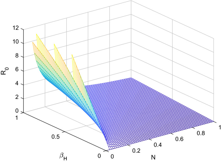
versus sensitive parameters and
Fig. 2.
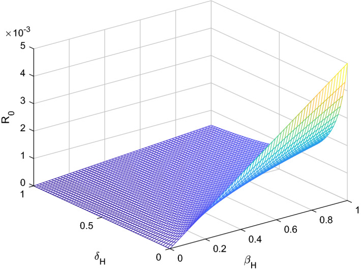
versus sensitive parameters and
Fig. 3.
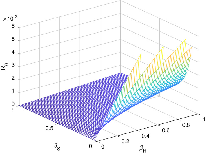
versus sensitive parameters and
Fig. 4.

versus sensitive parameters and
Fig. 5.
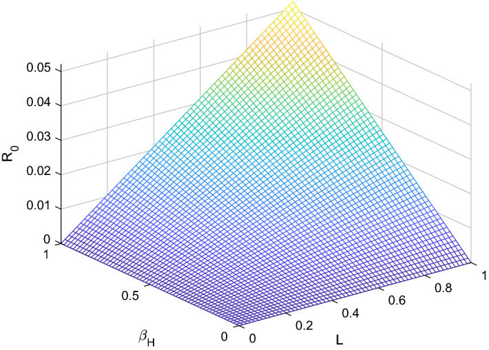
versus sensitive parameters and
Fig. 6.

versus sensitive parameters and
Discussions
In this section, we present the solution for the system (6) employing the Laplace-Adomian decomposition method (LADM). The fractional-order shows the realistic decline behavior of infection of disease. Therefore, here, the advantage of the fractional model is shown by the method of LADM on the various graphs. Let us take into account the following fractional system
| 45 |
with the initial conditions . Applying Laplace transform to both sides of the system (45), we have
| 46 |
By the definition of Caputo Laplace transform, it can be written
| 47 |
and so we reach
| 48 |
Let us assume that the solution S(t), H(t) and C(t) is in the form of infinite series as follows
| 49 |
The non-linear terms SH and SC involved in the system (45) are decomposed by Adomian polynomial as below
| 50 |
where and are Adomian polynomials. They are given by
| 51 |
The first six polynomials are as follows
| 52 |
and
| 53 |
Utilizing the (52) and (53), one can attain
| 54 |
| 55 |
and
| 56 |
by continuing in a similar manner, we get
| 57 |
Now applying inverse Laplace transformation on system (54), (55) and (56) we get
| 58 |
| 59 |
and
| 60 |
By using the parameter values in Table 2 when , and , the solution for three terms can be given by
| 61 |
In particular case let , so the solution after three terms is as below
| 62 |
Table 2.
Parameter values for the transmission dynamics of CA-MRSA and HA-MRSA obtained from the Beth Israel Deaconess Medical Center
| Parameter | Symbol | Baseline Value | Source |
|---|---|---|---|
| Total number of patients | 400 | [9] | |
| Length of stay | |||
| Susceptible | 5 days | [9] | |
| Colonized CA-MRSA | 7 days | [9] | |
| Colonized HA-MRSA | 5 days | [9] | |
| Transmission rate per susceptible individuals to | |||
| Colonized CA-MRSA per colonized CA-MRSA | 0.45 per day | [9] | |
| Colonized HA-MRSA per colonized HA-MRSA | 0.4 per day | [9] | |
| Decolonization rate per colonized patient per day per length of stay | |||
| CA-MRSA | 0.1 per day | [9] | |
| HA-MRSA | 0.1 per day | [9] | |
For analysis purposes in the present work, the values of the parameters are obtained from the Beth Israel Deaconess Medical Center and values of the fractional-order parameter are chosen differently as can be seen in the figures. Initial conditions are given for obtaining the solutions of fractional-order staph infection model (6) as [90, 80, 80]. The behavior of susceptible patients who are not colonized with HA-MRSA or CA-MRSA S(t) can be seen in Figs. 7, 8. Patients colonized with HA-MRSA H(t) and patients colonized with CA-MRSA C(t) can be seen in Figs. 9, 10, 11, 12, respectively. Also, the behavior of the solution curves of all three classes can be observed together in Fig. 13 when arbitrary order . Figures 7, 8, 9, 10, 11, 12 are depicted with the varying values of the fractional-order . The fractional and classical solution curves are shown separately for and . In this way, it can be understood that as the values approach 1, the solution curves approach the classical solution. It should be noted that the classical solution is represented by . For susceptible patients who are not colonized with HA-MRSA or CA-MRSA S(t), from Figs. 7 and 8, one can see that such choices of values indicate the decreasing rate for decreasing values of the fractional-order . When susceptible subclass S(t) decrease as in Figs. 7 and 8, the danger in the hospital will also get decreased due to the potential decrease in the infectious classes H(t) and C(t). As clearly seen, the choices of arbitrary order can bring about a strongly decreasing rate in S(t), which can be superb and better for the individuals in the hospital. For the patients colonized with HA-MRSA H(t), Figs. 9 and 10 affirm a decreasing rate with a slight form of the increasing rate as the values keep varying lower. On the other hand, Figs. 11 and 12 for the patients colonized with CA-MRSA behaves similarly. This is a well-motivated impact as the number of H(t) and C(t) get decreased vehemently with the decrease of the susceptible class S(t). Also, this is a realistic situation which suggests that if the S(t) decreases then its density would decrease and consequently the infected classes H(t) and C(t) would reduce at the speedier rate for smaller values of the fractional-order . Further observations affirm that for smaller values of , the stability for S(t), H(t) and C(t) does not take long duration as it does for .
Fig. 7.
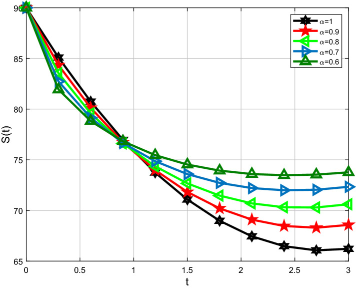
Comparison of Caputo and classical derivative for susceptible class S(t)
Fig. 8.

Comparison of Caputo and classical derivative for susceptible class S(t)
Fig. 9.
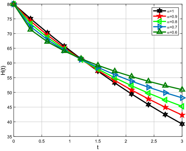
Comparison of Caputo and classical derivative for HA-MRSA class H(t)
Fig. 10.
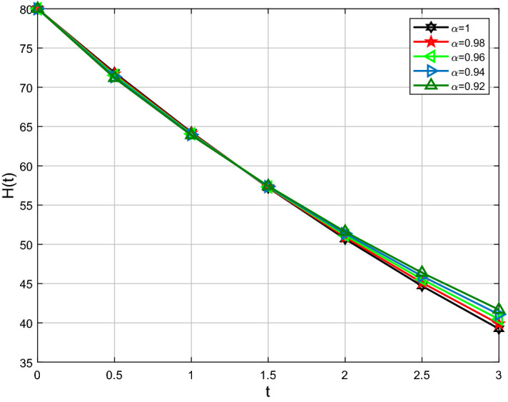
Comparison of Caputo and classical derivative for HA-MRSA class H(t)
Fig. 11.

Comparison of Caputo and classical derivative for CA-MRSA class C(t)
Fig. 12.
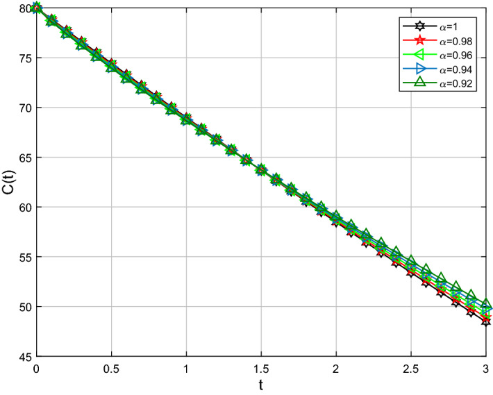
Comparison of Caputo and classical derivative for CA-MRSA class C(t)
Fig. 13.
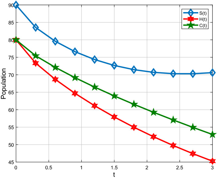
Comparison with Caputo derivative for S(t), H(t) and C(t) when
Concluding remarks
Some important conclusions that can be drawn from this study can be listed as follows:
The governing model has been proposed for the very first time under Caputo fractional operator. This fractional model (6) analyzes community-acquired and hospital-acquired methicillin-resistant Staphylococcus aures which when assuming different values of the fractional-order allowed us to observe the behavior of the solution curves in detail.
The key explanation for advantages of the non-local fractional derivatives is owing to the presence of many orders of freedom for the operators which is not possible in the classical case.
The current research is crucial since the model under consideration is of a non-linear type.
By employing the concept of fixed point theory, the existence and uniqueness of solutions have been achieved by Caputo fractional derivative.
Furthermore, the iterative solutions have been shown by utilizing the Laplace transform of Caputo fractional derivative. Also, the stability criteria for the fractional model (6) has also been presented by using the fixed point theorem.
On the other hand, the sensitivity analysis of the basic reproduction number of the aforementioned model has been carried out in order to determine the parameters that have the most crucial effect on the spread of the disease.
With the help of an efficient method of LADM, the numerical characteristics of the fractional model (6) have been depicted by the parameter values obtained from the Beth Israel Deaconess Medical Center.
Multifarious graphical diagrams in this study suggest that the introduced fractional model is sufficiently capable to the entire system.
Generally, it can be expressed that fractional models are thus not only an important tool for a more advantageous representation of the behavior of physical organisms and epidemiology but also capable of better prediction for ecosystems.
It should be noted that the main goal of the present work is to employ the LADM and see its effectiveness on the model under consideration. However, as a future direction, the proposed model can be analyzed by utilizing some other useful numerical methods and compared with each other.
Footnotes
Publisher's Note
Springer Nature remains neutral with regard to jurisdictional claims in published maps and institutional affiliations.
References
- 1.Brauer, F.: Compartmental models in epidemiology. In: Mathematical Epidemiology (pp. 19–79). Springer, Berlin (2008)
- 2.Byrne JP, editor. Encyclopedia of Pestilence, Pandemics, and Plagues. West Port: Greenwood Press; 2008. [Google Scholar]
- 3.Djuretic, T., Herbert, J., Drobniewski, F., Yates, M., Smith, E.G., Magee, J.G., Crowe, M.: Antibiotic resistant tuberculosis in the United Kingdom: 1993–1999. Thorax 57(6), 477–482 (2002) [DOI] [PMC free article] [PubMed]
- 4.Gruson, D., Hilbert, G., Vargas, F., Valentino, R., Bebear, C., Allery, A., Cardinaud, J.P.: Rotation and restricted use of antibiotics in a medical intensive care unit: impact on the incidence of ventilator-associated pneumonia caused by antibiotic-resistant gram-negative bacteria. Am. J. Respirat. Crit. Care Med. 162(3), 837–843 (2000) [DOI] [PubMed]
- 5.Hethcote HW. The mathematics of infectious diseases. SIAM Rev. 2000;42(4):599–653. doi: 10.1137/S0036144500371907. [DOI] [Google Scholar]
- 6.Joint United Nations Programme on HIV/AIDS. (2010). Global report: UNAIDS report on the global AIDS epidemic 2010. Unaids
- 7.Bernoulli D, Blower S. An attempt at a new analysis of the mortality caused by smallpox and of the advantages of inoculation to prevent it. Rev. Med. Virol. 2004;14(5):275. doi: 10.1002/rmv.443. [DOI] [PubMed] [Google Scholar]
- 8.Hamer WH. Epidemic Disease in England: The Evidence of Variability and of Persistency of Type. Bedford: Bedford Press; 1906. [Google Scholar]
- 9.Nagle, R.K., Saff, E.B., Snider, A.D.: Fundamentals of differential equations. Pearson Education (2014)
- 10.Qureshi S, Yusuf A. Modeling chickenpox disease with fractional derivatives:fFrom caputo to atangana-baleanu. Chaos Solitons Fract. 2019;122:111–118. doi: 10.1016/j.chaos.2019.03.020. [DOI] [Google Scholar]
- 11.Qureshi S, Yusuf A. Mathematical modeling for the impacts of deforestation on wildlife species using Caputo differential operator. Chaos Solitons Fract. 2019;126:32–40. doi: 10.1016/j.chaos.2019.05.037. [DOI] [Google Scholar]
- 12.Caputo M, Fabrizio M. A new definition of fractional derivative without singular kernel. Progr. Fract. Differ. Appl. 2015;1(2):1–13. [Google Scholar]
- 13.Atangana, A., Baleanu, D.: New fractional derivatives with nonlocal and non-singular kernel: theory and application to heat transfer model. arXiv preprint arXiv:1602.03408 (2016)
- 14.Baleanu D, Fernandez A. On fractional operators and their classifications. Mathematics. 2019;7(9):830. doi: 10.3390/math7090830. [DOI] [Google Scholar]
- 15.Yavuz M. Novel solution methods for initial boundary value problems of fractional order with conformable differentiation. Int. J. Optim. Control: Theories Appl. (IJOCTA) 2017;8(1):1–7. [Google Scholar]
- 16.Baleanu D, Fernandez A, Akgül A. On a fractional operator combining proportional and classical differintegrals. Mathematics. 2020;8(3):360. doi: 10.3390/math8030360. [DOI] [Google Scholar]
- 17.Qureshi S, Yusuf A, Shaikh AA, Inc M, Baleanu D. Fractional modeling of blood ethanol concentration system with real data application. Chaos: Interdiscip. J. Nonlinear Sci. 2019;29(1):013143. doi: 10.1063/1.5082907. [DOI] [PubMed] [Google Scholar]
- 18.Yusuf A, Inc M, Aliyu AI. On dark optical solitons of the space time nonlinear Schrödinger equation with fractional complex transform for Kerr and power law nonlinearities. J. Coupl. Syst. Multisc. Dyn. 2018;6(2):114–120. doi: 10.1166/jcsmd.2018.1154. [DOI] [Google Scholar]
- 19.Acay B, Bas E, Abdeljawad T. Fractional economic models based on market equilibrium in the frame of different type kernels. Chaos Solitons Fract. 2020;130:109438. doi: 10.1016/j.chaos.2019.109438. [DOI] [Google Scholar]
- 20.Acay B, Bas E, Abdeljawad T. Non-local fractional calculus from different viewpoint generated by truncated M-derivative. J. Comput. Appl. Math. 2020;366:112410. doi: 10.1016/j.cam.2019.112410. [DOI] [Google Scholar]
- 21.Bas, E., Acay, B., Ozarslan, R.: The price adjustment equation with different types of conformable derivatives in market equilibrium (2019)
- 22.Acay B, Ozarslan R, Bas E. Fractional physical models based on falling body problem. AIMS Math. 2020;5(3):2608. doi: 10.3934/math.2020170. [DOI] [Google Scholar]
- 23.D’Agata EM, Webb GF, Pressley J. Rapid emergence of co-colonization with community-acquired and hospital-acquired methicillin-resistant Staphylococcus aureus strains in the hospital setting. Math. Model. Nat. Phenomena. 2010;5(3):76–93. doi: 10.1051/mmnp/20105306. [DOI] [PMC free article] [PubMed] [Google Scholar]
- 24.Kilbas, A.A.A., Srivastava, H.M., Trujillo, J.J.: Theory and Applications of Fractional Differential Equations (Vol. 204). Elsevier, Amsterdam (2006)
- 25.Pressley J, D’Agata EM, Webb GF. The effect of co-colonization with community-acquired and hospital-acquired methicillin-resistant Staphylococcus aureus strains on competitive exclusion. J. Theor. Biol. 2010;264(3):645–656. doi: 10.1016/j.jtbi.2010.03.036. [DOI] [PMC free article] [PubMed] [Google Scholar]
- 26.Wang Z, Yang D, Ma T, Sun N. Stability analysis for nonlinear fractional-order systems based on comparison principle. Nonlinear Dyn. 2014;75(1–2):387–402. doi: 10.1007/s11071-013-1073-7. [DOI] [Google Scholar]
- 27.Naghipour A, Manafian J. Application of the Laplace Adomian decomposition and implicit methods for solving Burgers’ equation. TWMS J. Pure Appl. Math. 2015;6(1):68–77. [Google Scholar]
- 28.Shah K, Bushnaq S. Numerical treatment of fractional endemic disease model via Laplace Adomian decomposition method. J. Sci. Arts. 2017;17(2):257. [Google Scholar]
- 29.Akinlar MA, Tchier F, Inc M. Chaos control and solutions of fractional-order Malkus waterwheel model. Chaos Solitons Fract. 2020;135:109746. doi: 10.1016/j.chaos.2020.109746. [DOI] [Google Scholar]
- 30.Qureshi S, Yusuf A, Ali Shaikh A, Inc M, Baleanu D. Mathematical modeling for adsorption process of dye removal nonlinear equation using power law and exponentially decaying kernels. Chaos: Interdiscip. J. Nonlinear Sci. 2020;30(4):043106. doi: 10.1063/1.5121845. [DOI] [PubMed] [Google Scholar]
- 31.Van den Driessche P, Watmough J. Reproduction numbers and sub-threshold endemic equilibria for compartmental models of disease transmission. Math. Biosci. 2002;180(1–2):29–48. doi: 10.1016/S0025-5564(02)00108-6. [DOI] [PubMed] [Google Scholar]
- 32.Haq, F., Shah, K., ur Rahman, G., Shahzad, M.: Numerical solution of fractional order smoking model via laplace Adomian decomposition method. Alexandria Eng. J. 57(2), 1061–1069 (2018)
- 33.Farman M, Saleem MU, Ahmad A, Ahmad MO. Analysis and numerical solution of SEIR epidemic model of measles with non-integer time fractional derivatives by using Laplace Adomian Decomposition Method. Ain Shams Eng. J. 2018;9(4):3391–3397. doi: 10.1016/j.asej.2017.11.010. [DOI] [Google Scholar]
- 34.Sweilam, N. H., AL-Mekhlafi, S. M., Albalawi, A. O.: Optimal control for a fractional order malaria transmission dynamics mathematical model. Alexandria Eng. J. (2020)
- 35.Sweilam NH, Al-Mekhlafi SM, Albalawi AO, Baleanu D. On the optimal control of coronavirus (2019-nCov) mathematical model; a numerical approach. Adv. Differ. Equ. 2020;2020(1):1–13. doi: 10.1186/s13662-019-2438-0. [DOI] [PMC free article] [PubMed] [Google Scholar]
- 36.Sweilam, N. H., Al-Mekhlafi, S. M., & Baleanu, D.: A hybrid fractional optimal control for a novel Coronavirus (2019-nCov) mathematical model. J. Adv. Res. (2020) [DOI] [PMC free article] [PubMed]
- 37.Djilali S, Ghanbari B, Bentout S, Mezouaghi A. Turing-Hopf bifurcation in a diffusive mussel-algae model with time-fractional-order derivative. Chaos Solitons Fract. 2020;138:109954. doi: 10.1016/j.chaos.2020.109954. [DOI] [Google Scholar]
- 38.Soufiane B, Touaoula TM. Global analysis of an infection age model with a class of nonlinear incidence rates. J. Math. Anal. Appl. 2016;434(2):1211–1239. doi: 10.1016/j.jmaa.2015.09.066. [DOI] [Google Scholar]
- 39.Djilali, S., Bentout, S.: Spatiotemporal patterns in a diffusive predator-prey model with prey social behavior. Acta Applicandae Mathematicae 1–19 (2019)
- 40.Ghanbari B, Djilali S. Mathematical and numerical analysis of a three-species predator-prey model with herd behavior and time fractional-order derivative. Math. Methods Appl. Sci. 2020;43(4):1736–1752. doi: 10.1002/mma.5999. [DOI] [Google Scholar]
- 41.Souna F, Djilali S, Charif F. Mathematical analysis of a diffusive predator-prey model with herd behavior and prey escaping. Math. Model. Nat. Phenomena. 2020;15:23. doi: 10.1051/mmnp/2019044. [DOI] [Google Scholar]
- 42.Djilali S. Pattern formation of a diffusive predator-prey model with herd behavior and nonlocal prey competition. Math. Methods Appl. Sci. 2020;43(5):2233–2250. doi: 10.1002/mma.6036. [DOI] [Google Scholar]
- 43.Djilali S. Effect of herd shape in a diffusive predator-prey model with time delay. J. Appl. Anal. Comput. 2019;9(2):638–654. [Google Scholar]


