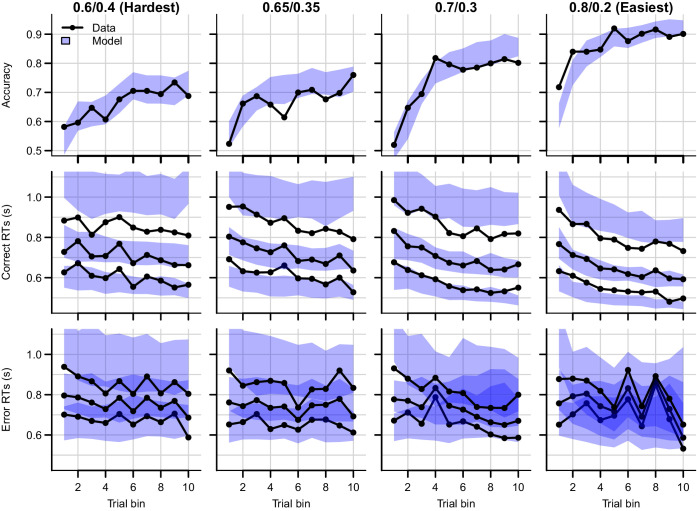
Figure 4. Data (black) and posterior predictive distribution of the RL-ARD (blue), separately for each difficulty condition.

Column titles indicate the reward probabilities, with 0.6/0.4 being the most difficult, and 0.8/0.2 the easiest condition. Top row depicts accuracy over trial bins. Middle and bottom rows show 10th, 50th, and 90th RT percentiles for the correct (middle row) and error (bottom row) response over trial bins. Shaded areas correspond to the 95% credible interval of the posterior predictive distributions. All data and fits are collapsed across participants.

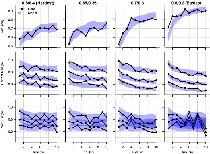
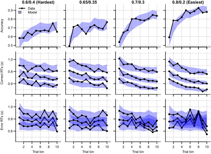
Figure 4—figure supplement 1. Data (black) and posterior predictive distribution of the RL-DDM (blue), separately for each difficulty condition.

Row titles indicate the reward probabilities, with 0.6/0.4 being the most difficult, and 0.8/0.2 the easiest condition. Top row depicts accuracy over trial bins. Middle and bottom row illustrate 10th, 50th, and 90th quantile RT for the correct (middle row) and error (bottom row) response over trial bins. Shaded areas correspond to the 95% credible interval of the posterior predictive distributions. All data are collapsed across participants.

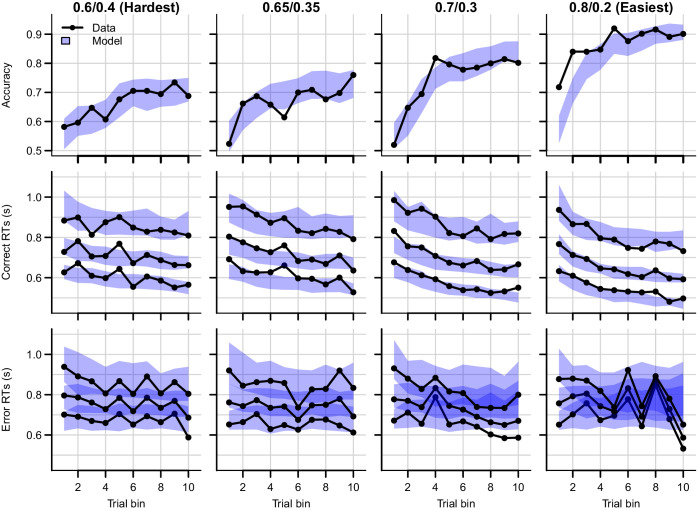
Figure 4—figure supplement 2. Data (black) and posterior predictive distribution of the RL-ARD (blue), separately for each difficulty condition, excluding 17 subjects which had perfect accuracy in the first bin of the easiest condition.

Row titles indicate the reward probabilities, with 0.6/0.4 being the most difficult, and 0.8/0.2 the easiest condition. Top row depicts accuracy over trial bins. Middle and bottom row illustrate 10th, 50th, and 90th quantile RT for the correct (middle row) and error (bottom row) response over trial bins. Shaded areas correspond to the 95% credible interval of the posterior predictive distributions. All data are collapsed across participants.

Figure 4—figure supplement 3. Posterior predictive distribution of the RL-ALBA model on the data of experiment 1, with one column per difficulty condition.

The LBA assumes that, on every trial, two accumulators race deterministically toward a common bound b. Each accumulator i starts at a start point sampled from a uniform distribution [0, A], and with a speed of evidence accumulation sampled from a normal distribution $\mathcal{𝒩}\left(v_i,s_i\right)$. In the RL-ALBA model, we used Equation 4 to link Q-values to LBA drift rates $v_1$ and $v_2$ (excluding the $sW$ term, since the LBA assumes no within-trial noise). Instead of directly estimating threshold b, we estimated the difference B = b-A (which simplifies enforcing b>A). We used the following mildly informed priors for the hypermeans: $V_0~\mathcal{𝒩}\left(2,5\right)$, $w_d~\mathcal{𝒩}\left(9,5\right)$ truncated at lower bound 0, $w_s~\mathcal{𝒩}\left(0,3\right)$, $s_2~\mathcal{𝒩}\left(1,1\right)$, $A~\mathcal{𝒩}\left(1,1\right)$, $B~\mathcal{𝒩}\left(3,5\right)$ truncated at lower bound 0, and $t_0~\mathcal{𝒩}\left(0.3,0.5\right)$, truncated at lower bound 0.025 and upper bound 1. For the hyperSDs, all priors were $\mathrm{\Gamma }(1,\mathrm{}1)$. The summed BPIC was 4836, indicating that the RL-ALBA performs slightly better than the RL-DDM with between-trial variabilities (BPIC = 4844), and better than the RL-lARD (BPIC = 4849), but not as well as the RL-ARD (BPIC = 4577).

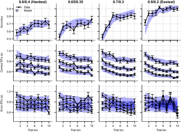
Figure 4—figure supplement 4. Data (black) and posterior predictive distribution of the RL-ARD (blue), separately for each difficulty condition.

Column titles indicate the reward probabilities, with 0.6/0.4 being the most difficult, and 0.8/0.2 the easiest condition. Top row depicts accuracy over trial bins. Middle and bottom rows show 10th, 50th, and 90th RT percentiles for the correct (middle row) and error (bottom row) response over trial bins. Shaded areas correspond to the 95% credible interval of the posterior predictive distributions. All data and fits are collapsed across participants. Error bars depict standard errors.