The analysis of isolation measures for epidemic control of COVID-19

Abstract

This paper proposes a susceptible exposed infectious recovered model (SEIR) with isolation measures to evaluate the COVID-19 epidemic based on the prevention and control policy implemented by the Chinese government on February 23, 2020. According to the Chinese government’s immediate isolation and centralized diagnosis of confirmed cases, and the adoption of epidemic tracking measures on patients to prevent further spread of the epidemic, we divide the population into susceptible, exposed, infectious, quarantine, confirmed and recovered. This paper proposes an SEIR model with isolation measures that simultaneously investigates the infectivity of the incubation period, reflects prevention and control measures and calculates the basic reproduction number of the model. According to the data released by the National Health Commission of the People’s Republic of China, we estimated the parameters of the model and compared the simulation results of the model with actual data. We have considered the trend of the epidemic under different incubation periods of infectious capacity. When the incubation period is not contagious, the peak number of confirmed in the model is 33,870; and when the infectious capacity is 0.1 times the infectious capacity in the infectious period, the peak number of confirmed in the model is 57,950; when the infectious capacity is doubled, the peak number of confirmed will reach 109,300. Moreover, by changing the contact rate in the model, we found that as the intensity of prevention and control measures increase, the peak of the epidemic will come earlier, and the peak number of confirmed will also be significantly reduced. Under extremely strict prevention and control measures, the peak number of confirmed cases has dropped by nearly 50%. In addition, we use the EEMD method to decompose the time series data of the epidemic, and then combine the LSTM model to predict the trend of the epidemic. Compared with the method of directly using LSTM for prediction, more detailed information can be obtained.

Introduction

After the outbreak of the novel coronavirus pneumonia (COVID-19), the Chinese government quickly adopted relevant anti-epidemic measures, effectively curbing the development of the domestic epidemic. In other countries, the epidemic situation is still on the rise due to the lack of effective measures. According to data released by the World Health Organization(https://covid19.who.int/table), as of 14:22 on December 27, 2020, Central European Time, the number of confirmed coronavirus cases worldwide increased by 434,779 compared with the previous day, reaching 79,232,555 cases. The number of deaths increased by 7,393 compared with the previous day, reaching 1,754,493 cases. And the cumulative number of confirmed cases in the United States exceeded 18 million, and the cumulative number of deaths reached 328,014.

The recent movement of domestic workers who have resumed work has increased the risk of transmission, posing a considerable challenge to epidemic control. To scientifically guide epidemic prevention and control, it is necessary to establish a suitable model. At present, the SIS, SIR and SEIR models [1–3] provide a good way for the simulation of epidemics. It shows that those SIS, SIR and SEIR models can reflect the dynamics of different epidemics well. Meanwhile, these models have been used to model the COVID-19. For instance, He Shaobo et al. [4] proposed a SEIR epidemic model for the COVID-19 according to some general control strategies, such as hospital, quarantine and external input. And they estimated the model parameters through the particle swarm optimization (PSO) algorithm based on the epidemic data of Hubei Province. Iwata Kentaro and Miyakoshi Chisato [5] estimated the impact of potential secondary epidemics in the community through a random SEIR model. It found that in the worst case, the total number of people who will recover or transfer at 100 days is 997, the maximum number of symptomatic infectious disease patients per day is 335, and the average basic reproduction number is 6.5. Joseph Wu and Kathy Leung et al. [6] used data on the number of cases exported from Wuhan internationally from December 31, 2019 to January 28, 2020, to predict the development of the epidemic in Wuhan and predicted the spread of COVID-19 throughout the country and around the world. It has been proposed that the epidemic situation has increased exponentially in many major cities in China, while the time of the outbreak in Wuhan lags by approximately 1-2 weeks. Wang and Tang et al. [7] constructed a complex network model of COVID-19 propagation in Wuhan and surrounding 15 severely epidemic cities based on COVID-19 epidemic report data and large data on population migration and distribution. It proposed the possible time for resumption of labour in Wuhan and surrounding areas and the impact of nodes and resuming work on the risk of secondary outbreaks. And there are many other methods [8–14] used to study the epidemic trend of COVID-19.

The current epidemic situation shows that different types of infected persons require different prevention and control measures, and the effects of model fitting and epidemic prediction are different. For this reason, this paper considers the characteristics of isolation measures and incubation period that the infected persons are difficult to detect and contagious, divides the population into susceptible, exposed, infectious, quarantine, confirmed and recovered, and establishes an SEIR model with isolation measures.

SEIR epidemic model based on isolation measures

Model introduction

Based on epidemiological theory [15–19], the transmission characteristics of COVID-19 and the current isolation and control measures in China, the population at time t is now divided into susceptible, exposed, infectious, quarantine, confirmed and recovered. The susceptible individuals are not infected with the COVID-19 virus. The exposed individuals are infected with COVID-19 without showing obvious pathological features. The infectious individuals show pathological features and are highly contagious, but have not been isolated for the time being. The quarantine individuals are the incubation period patients who are isolated according to the epidemic tracking measures. The confirmed individuals are diagnosed with COVID-19 and isolated from the outside population. The recovered individuals are recovered after medical treatment. In this paper, we only consider human-to-human transmission, and the recent cold chain transmission has not been included in the investigation. And the probability of re-infection in recovered patients is very small.

The susceptible individuals may be infected and become the new individuals in the exposed group as long as they come into contact with virus carriers, i.e., the individuals in the exposed and infectious groups [20, 21]. According to the epidemic tracking measures, some exposed individuals will be isolated into the quarantine. And the quarantine will eventually be diagnosed as the confirmed after pathological examination. However, due to the complexity of crowd movement, some exposed individuals will gradually develop into the infectious without being isolated. The infectious individuals with obvious pathological features will be diagnosed in time to enter the confirmed class. The confirmed individuals will be cured after medical care and enter into the recovered. According to the abovementioned epidemic spread process and mechanism, the infectious process is further subdivided, and the quarantine class is added to obtain the SEIR epidemic model with isolation measures, which are defined as follows [22, 23]:

$$\left\{\begin{array}{cc}\frac{d{S}_t}{dt}& =\mu N_t-\beta c(I_t+k{E}_t)-\mu S_t\\ \frac{d{E}_t}{dt}& =\beta c(I_t+k{E}_t)-(t_{ei}+t_{eq}+\mu )E_t\\ \frac{d{I}_t}{dt}& =t_{ei}{E}_t-(t_{ic}+{\mu }_1+\mu )I_t\\ \frac{d{C}_t}{dt}& =t_{ic}{I}_t+t_{qc}{Q}_t-(\gamma +{\mu }_2+\mu )C_t\\ \frac{d{Q}_t}{dt}& =t_{eq}{E}_t-(t_{qc}+\mu )C_t\\ \frac{d{R}_t}{dt}& =\gamma C_t-\mu R_t\end{array}\right)$$ 1

The meanings of parameters in (1) are as follows:

• β denotes the standard infection rate of infectious, c denotes the expectation of the number of susceptible contacted by infectious or exposed. βc denotes the standard infection rate of infectious individuals

• k denotes the ratio of the standard infection rate of the infectious and exposed individuals.

• t_ei denotes the probability of conversion of exposed to infectious.

• t_eq denotes the probability of conversion of exposed to quarantine.

• t_qc denotes the probability of conversion of quarantine to confirmed.

• t_ic denotes the probability of conversion of infectious to confirmed.

• The cure rate of confirmed is γ.

• The mortality rate of infectious is μ₁. The mortality rate of confirmed is μ₂. The natural mortality rate is μ.

The basic reproduction number and equilibrium point of the model

The basic reproduction number is an important indicator to describe the incidence of infectious diseases. It refers to the expectation of the number of new infections caused by an infected person in an infectious time after entering a completely disease-free and susceptible population. If R₀ < 1, that is, the number of people infected by an infected person during the infection period is less than one on average, then the disease cannot spread among the population and eventually tends to die out. Conversely, if R₀ > 1, that is, the average number of people infected by an infected person exceeds one, the disease will continue to spread and become endemic [24].

To study the evolution of populations over time, we explore the stability of equilibrium states through the stability theory of differential equations without solving differential equations. In this paper, according to the approach reported in the literature [25, 26], each population type in the model is seen as a node in the network, the transformation of different population types are seen as connections between nodes, and the degree distribution of each node is uniform. Therefore, it can be seen as an infectious disease model on a uniform network, where the root of the model equation is called the disease-free equilibrium point when the rate of change in population size in the equation set of the infectious disease model is zero. The basic reproduction number R₀ of the model in this paper is then derived from the reproduction matrix at the disease-free equilibrium point, and the existence of the equilibrium point is analysed.

According to the set of equations, we only care about the information of exposed, infectious, quarantine, confirmed and recovered. Therefore, it is only necessary to consider the stability of the last five equations of the model, so that the original (1) can be written as (2):

$$\left\{\begin{array}{cc}\frac{d{E}_t}{dt}& =\beta c(I_t+k{E}_t)-(t_{ei}+t_{eq}+\mu )E_t\\ \frac{d{I}_t}{dt}& =t_{ei}{E}_t-(t_{ic}+{\mu }_1+\mu )I_t\\ \frac{d{C}_t}{dt}& =t_{ic}{I}_t+t_{qc}{Q}_t-(\gamma +{\mu }_2+\mu )C_t\\ \frac{d{Q}_t}{dt}& =t_{eq}{E}_t-(t_{qc}+\mu )Q_t\end{array}\right)$$ 2

First, we take X = (E,I,C,Q)^T and solve (3):

$$\left\{\begin{array}{cc}\beta c(I+kE)-(t_{ei}+t_{eq}+\mu )E& =0\\ t_{ei}E-(t_{ic}+{\mu }_1+\mu )I& =0\\ t_{ic}I+t_{qc}Q-(\gamma +{\mu }_2+\mu )C& =0\\ t_{eq}E-(t_{qc}+\mu )Q& =0\end{array}\right)$$ 3

It can be shown that (3) has one and only one possible solutions. The solution is the disease-free equilibrium point X₀ = (E₀,I₀,C₀,Q₀)^T = (0,0,0,0)^T.

Then, (2) can be written as follows:

$$\frac{dX}{dt}=F_{1234}\left(X\right)-V_{1234}\left(X\right)$$ 4

Among them,

$$F_{1234}\left(X\right)=\left\{\begin{array}{c}\beta c(I+kE)\\ 0\\ 0\\ 0\end{array}\right\},$$ 5

$$V_{1234}\left(X\right)=\left\{\begin{array}{c}(t_{ei}+t_{eq}+\mu )E\\ -t_{ei}E+(t_{ic}+{\mu }_1+\mu )I\\ -t_{ic}I+(\gamma +{\mu }_2+\mu )C-t_{qc}Q\\ -t_{eq}E+(t_{qc}+\mu )Q\end{array}\right\}\mathrm{.}$$ 6

Because X₀ is the disease-free equilibrium point of (4), so there is:

$$F=D{F}_{1234}{|}_{X=X_0}=\left\{\begin{array}{cccc}\beta ck& \beta c& 0& 0\\ 0& 0& 0& 0\\ 0& 0& 0& 0\end{array}\right\},$$ 7

$$V=D{V}_{1234}{|}_{X=X_0}=\left\{\begin{array}{cccc}{t}_{ei}+t_{eq}+\mu & 0& 0& 0\\ -t_{ei}& t_{ic}+{\mu }_1+\mu & 0& 0\\ 0& -t_{ic}& \gamma +{\mu }_2+\mu & -t_{qc}\\ -t_{eq}& 0& 0& t_{qc}+\mu \end{array}\right\}\mathrm{.}$$ 8

The reproduction matrix can be obtained as follows:

$$F{V}^{-1}=\left\{\begin{array}{cccc}\frac{\beta c\left(k\right(t_{ic}+{\mu }_1+\mu )+t_{ei})}{(t_{ei}+t_{eq}+\mu )(t_{ic}+{\mu }_1+\mu )}& \frac{\beta c}{t_{ic}+{\mu }_1+\mu }& 0& 0\\ 0& 0& 0& 0\\ 0& 0& 0& 0\end{array}\right\}$$ 9

Therefore, the basic reproduction number R₀ = ρ(FV^− 1), which is the spectral radius of FV^− 1, can now be derived:

$$R_0=\frac{\beta c\left(k\right(t_{ic}+{\mu }_1+\mu )+t_{ei})}{(t_{ei}+t_{eq}+\mu )(t_{ic}+{\mu }_1+\mu )}$$ 10

The expression of the basic reproduction number R₀ is divided into two terms: $\frac{1}{t_{ei}+t_{eq}+\mu }$ is the average length of the incubation period, $\beta ck\frac{1}{t_{ei}+t_{eq}+\mu }$ is the average number of people who can be infected during an incubation period, $\frac{1}{t_{ic}+{\mu }_1+\mu }$ is the average length of the infectious period, and $\frac{t_{ei}}{t_{ei}+t_{eq}+\mu }$ is the proportion of patients in the incubation period entering the infectious period. $\beta c\frac{t_{ei}}{(t_{ei}+t_{eq}+\mu )(t_{ic}+{\mu }_1+\mu )}$ represents the average number of patients who can be infected during the infection period, which meets the definition of basic reproduction number.

Stability of disease-free equilibrium points

The Jacobian matrix at the disease-free equilibrium point X₀ in (2) is:

$$\left\{\begin{array}{cccc}\beta ck-(t_{ei}+t_{eq}+\mu )& \beta c& 0& 0\\ t_{ei}& -(t_{ic}+{\mu }_1+\mu )& 0& 0\\ 0& t_{ic}& -(\gamma +{\mu }_2+\mu )& t_{qc}\\ t_{eq}& 0& 0& -(t_{qc}+\mu )\end{array}\right\}$$ 11

The corresponding characteristic polynomial is:

$$\begin{array}{rcl}|\lambda E-J|& =& \left|\begin{array}{cccc}\lambda -\beta ck+t_{ei}+t_{eq}+\mu & -\beta c& 0& 0\\ -t_{ei}& \lambda +t_{ic}+{\mu }_1+\mu & 0& 0\\ 0& -t_{ic}& \lambda +\gamma +{\mu }_2+\mu & -t_{qc}\\ -t_{eq}& 0& 0& \lambda +t_{qc}+\mu \end{array}\right|\\ & =& (\lambda +\gamma +{\mu }_2+\mu )(\lambda +t_{qc}+\mu )\left|\begin{array}{cc}\lambda -\beta ck+t_{ei}+t_{eq}+\mu & -\beta c\\ -t_{ei}& \lambda +t_{iq}+{\mu }_1+\mu \end{array}\right|\\ & =& (\lambda +\gamma +{\mu }_2+\mu )(\lambda +t_{qc}+\mu )({\lambda }^2+a_1\lambda +a_2)\end{array}$$ 12

To simplify symbols, a₁ = (t_ic + μ₁ + μ) + (t_ei + t_eq + μ − βck), a₂ = (t_ic + μ₁ + μ)(t_ei + t_eq + μ − βck) − βct_ei.

According to the first two factors, $\left|\begin{array}{c}\lambda E-J\end{array}\right|=0$ has the following two negative roots, i.e., λ₁ = −(γ + μ₂ + μ), λ₂ = −(t_qc + μ). Moreover, by the Routh-Hurwitz Criteria, to allow the root of λ² + a₁λ + a₂ to have a negative real part, we need to ensure a₁ > 0, $\left|\begin{array}{cc}{a}_1& 0\\ 1& a_2\end{array}\right|>0$, to conclude that:

$$\frac{\beta c\left(k\right(t_{ic}+{\mu }_1+\mu )+t_{ei})}{(t_{ei}+t_{eq}+\mu )(t_{ic}+{\mu }_1+\mu )}=R_0<1$$ 13

Therefore, for the model described in (2), when R₀ < 1, the disease-free equilibrium point X₀ is globally asymptotically stable; when R₀ > 1, the disease-free equilibrium point X₀ is unstable.

Improved LSTM model based on ensemble empirical mode decomposition

In order to extract the eigenvalues of the time series data of the COVID-19 epidemic, this paper adopts the Ensemble Empirical Mode Decomposition (EEMD) method, which is based on the Empirical Mode Decomposition (EMD) method by adding Gaussian white noise with the same intensity but different sequences to supplement the missing signal, and perform the new signal break down [27]. The process of EEMD method to extract characteristic signals is as follows:

Step 1: Add Gaussian white noise 𝜖(t) to the original signal x(t):

$$X\left(t\right)=x\left(t\right)+𝜖\left(t\right)$$ 14

Step 2: Decompose X(t) into intrinsic mode function (IMF) components by EMD:

$$X\left(t\right)=\sum _{j=1}^n{h}_j\left(t\right)+r_n\left(t\right)$$ 15

Among them, h_j(t) is the j-th IMF component after decomposition of X(t), r_n(t) is the residual after decomposition of X(t), n is the number layers of decomposition.

Step 3: Each time a different Gaussian white noise 𝜖_i(t)(i = 1,2,⋯ ,n) is added to x(t), step 1 and step 2 are repeated to obtain a different noise-containing signal X_i(t) = x(t) + 𝜖_i(t), which is decomposed into:

$$X_i\left(t\right)=\sum _{j=1}^n{h}_{ij}+r_{in}$$ 16

Step 4: The average of all IMF components obtained in step 3 is used as the final result of decomposition:

$$h_j^{‘}\left(t\right)=\frac{1}{n}\sum _{j=1}^n{h}_{ij}\left(t\right)$$ 17

Among them, $h_j^{‘}\left(t\right)$ is the j-th IMF component of original signal x(t) after the decomposition of EEMD.

We have obtained six IMF components of the COVID-19 epidemic sequence, which represent the characterization of the original signal from different aspects. Then, we use the obtained IMF signal components as features in different aspects, and each IMF signal component is passed through a long-short time memory (LSTM) network, and finally the weighted sum of the output of each LSTM network is used as the prediction result.

Simulation results

This section analyses the actual situation according to the literature [28, 29], combines the simulation results of the model, and compares the simulation results of the model with the actually reported occurrences. Moreover, we were inspired by other methods [30] and tried to predict the epidemic through improved LSTM models based on ensemble empirical mode decomposition.

The estimation of parameter

The real epidemic data used in this paper come from the National Health Commission of the People’s Republic of China(http://www.nhc.gov.cn/xcs/yqtb/list_gzbd.shtml). We crawled the daily real-time data published on the website and selected the data at the same time point each day as the research data set after aggregating. Parameter assignment refers to the Diagnosis and Treatment Protocol for COVID-19 (5 Edition Trial) issued by the National Health Commission (NHC) on February 5, 2020 and literature [31]. However, the literature does not consider the infectivity of patients during the incubation period and overestimates the infection rate. Moreover, the formal prevention and control measures started on January 23, 2020, and the contact rate between personnel was relatively stable. Therefore, this paper adjusted the probability of contact infection and based the probability on more current raw data to compare the other parameters, which are fitted and optimized to improve the model prediction accuracy. Because the incubation period of COVID-19 has been reported to be between 2 and 14 days, we chose the midpoint of 7 days. According to the epidemic tracking measures, we found that nearly 80% of the population will become quarantine class, and the rest will become the infectious class. So we set t_eq = 0.114, t_ei = 0.0286. In addition, the infectious individual with obvious pathological feature and the quarantine will be diagnosed and isolated in about three days, so we set t_ic = t_qc = 0.333. The mortality rate of confirmed is μ₂ = 3.17% according to the actual data, and we estimated the mortality rate of infectious is μ₁ = 6.34% and the cure rate is γ = 3.33%.

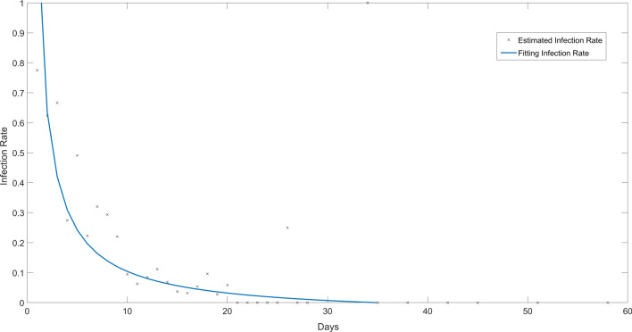
We estimated the infection rate of Infectious through the number of newly confirmed diagnoses every day, that is, the number of people infected by each Infectious individual every day. According to the previous data, we set the incubation period of Exposed to 7 days, and the Infectious will be diagnosed and isolated in about 3 days. We estimate the number of Infectious at time t by the number of newly confirmed diagnoses from t − 10 to t − 8, and the number of newly confirmed diagnoses at time t − 7 to t − 1 is the number of Exposed at time t. According to the above considerations, we use the data of newly confirmed patients in Hubei Province from February 17 to May 29 to obtain the infection rate of Infectious changing over time as β(t) = 1.309t^− 0.9384 − 0.04684, and the fitted curve is shown in Fig. 1.

Fig. 1.

The Fitting Result of Infection Rate of Infectious

The impact of infectious capability during the incubation period

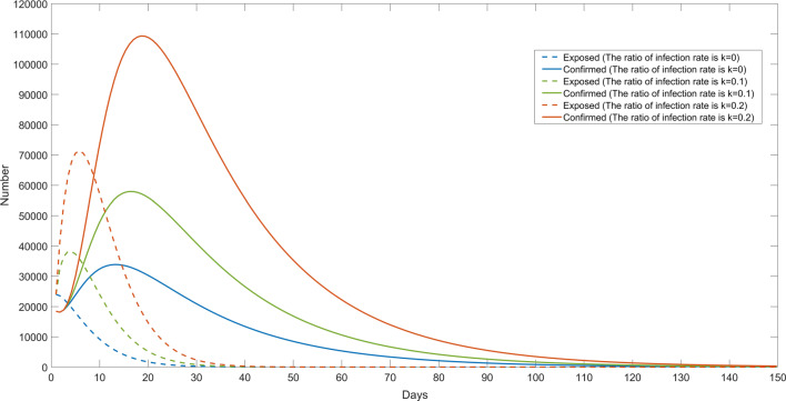
Considering the impact of infectivity during the incubation period on the epidemic trend, we simulated the trend of the epidemic in different situations by adjusting the value of k, which represents the ratio of infectivity during the incubation period to the infectious period in our model, and the simulation results are shown in Fig. 2. When k = 0, that is, the incubation period is not contagious, the peak number of confirmed is 33,870; when k = 0.1, the peak number of confirmed is 57,950; when k = 0.2, the peak number of confirmed reaches 109,300. By comparing the trend of the actual curve change in the epidemic, the model that considers the infectious incubation period is more realistic.

Fig. 2.

The Simulation Results with Different Infectivity in the Incubation Period

The epidemic trend under different contact rates

According to the Level I response of public health emergencies initiated by Hubei on January 24, 2020, necessary prevention and control isolation measures have been undertaken, e.g., limiting or stopping crowd gathering activities such as fairs, assemblies, and cinemas, and taking preventive measures against the floating population to prevent the spread of the virus among people. These measures are equivalent to controlling the number of susceptible persons contacted by virus carriers in this model. We simulated the epidemic under different levels of prevention and control measures by changing the numerical value of the contact rate.

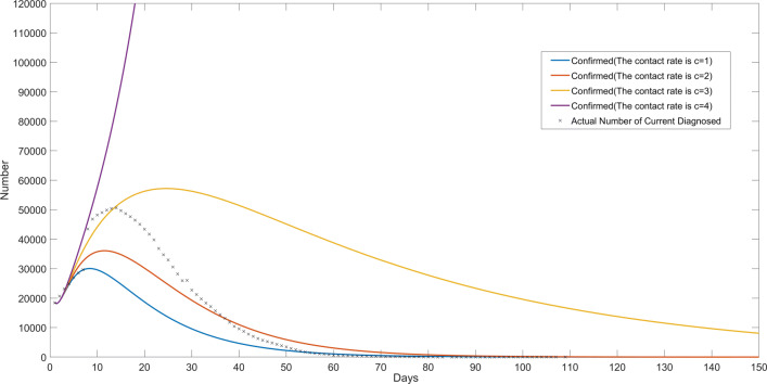
In order to simplify the discussion, we selected a suitable fixed standard infection rate β = 0.24, and then simulated the epidemic trend when the contact rate is c = 1, c = 2, c = 3, and c = 4, respectively, and the simulation results are shown in Fig. 3. In addition, we separately calculated the basic reproduction number R₀ in the corresponding situation. When c = 1, it means that the prevention and control is extremely strict, and the corresponding basic reproduction number is R₀ = 0.3089, and the peak number of confirmed patients is only about 30,040. When c = 2, the corresponding basic reproduction number is R₀ = 0.6178, and the peak number of confirmed patients is approximately 30,040. When c = 3, the corresponding basic reproduction number is R₀ = 0.9267, and the peak number of confirmed patients is 57,080, which is close to the actual value. When c = 4, it reflects the situation when the prevention and control measures are not in place, and the corresponding basic reproduction number is R₀ = 1.2356. At this time, the number of confirmed cases shows a trend of dispersion. It can be seen that the intensity of prevention and control measures plays an important role in curbing the development of the epidemic. With the increase in the intensity of prevention and control measures, the peak number of confirmed cases will gradually decrease, and it will help to reach the peak point earlier. Under extremely strict prevention and control measures, the peak number of confirmed cases has dropped by nearly 50%. In addition, we can see that when the basic reproduction number R₀ < 1, as shown in Fig. 3 when c = 1,2,3, the model gradually converges. Moreover, the smaller the value of R₀, the fewer the number of single virus carriers infects, the faster the convergence of the model. When R₀ > 1, the model will diverge, as shown in Fig. 3 when c = 4, the epidemic will continue to spread.

Fig. 3.

The Simulation Results under Different Contact Rates

Comparison of simulation results and the actual data

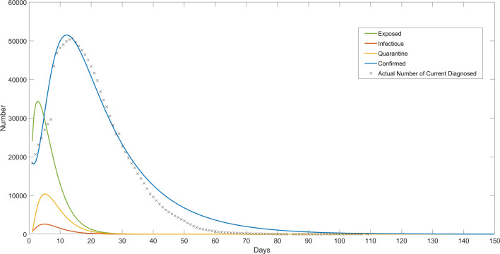
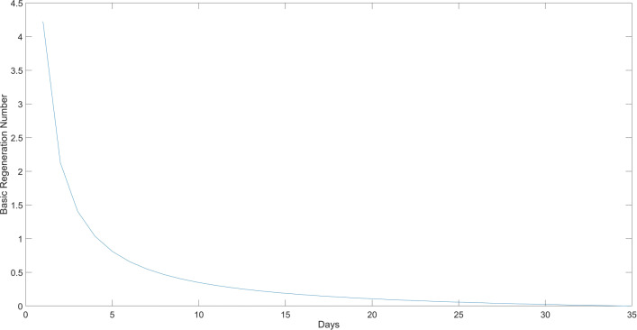
In this paper, based on the SEIR model, we further consider the fact that the actual epidemic control has considered the intensive screening of the patients and the strict isolation of the confirmed patients. By doing so, the patients in the infectious period in the original SEIR model are partially isolated and can no longer participate in the transmission of the virus. The simulation results of the model proposed in this paper are shown in Fig. 4. The black spots are the actual number of current diagnosed in Hubei Province from February 6, 2020, to May 29, 2020. And according to the fitting result, the change of the basic reproduction number R₀ is shown in Fig. 5. The simulated trend of the confirmed class is consistent with the actually reported occurrences.

Fig. 4.

The Simulation Results of the SEIR Model Based on Isolation Measures

Fig. 5.

The Change of Basic Reproduction Number R₀

The simulation results of SIR model

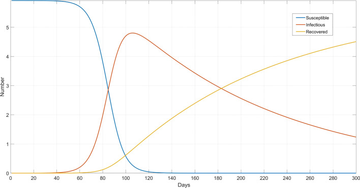
We can make further simulations by using the SIR model, that is, considering that the infected may be objectively immune after recovery. Although again there is no conclusive evidence to prove that persons cured in this epidemic outbreak have immunity, based on the control measures of this epidemic, the recovered may be considered to some extent that they are protected in intact isolation, which makes re-infection rare. Hence, they may be identified as a separate type of complete withdrawal from the infection system, as the curve shown in Fig. 6.

Fig. 6.

The Simulation Results of SIR Model

The simulation results of the logistic model

In this paper, we also attempted to simulate the epidemic through the logistic model. The logistic model is a common sigmoid function that is widely used in the simulation of biological reproduction and growth processes and population growth processes.

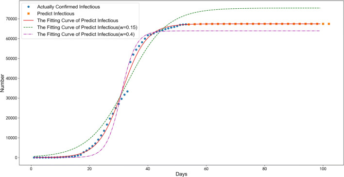
According to the nature of the logistic model, the greater the growth rate ω in the model, the faster it reaches the limit value M(namely, the maximum number of infected people). In this paper, the logistic model is used to fit the number of confirmed infections from January 1, 2020, to March 3, 2020, by nonlinear least squares. According to the principle of minimizing the mean square error, grid tuning is used to find the optimal parameters, the (10,000,90,000) interval is traversed with a step length of 1 for the model limit M, and the (0,1) interval is traversed with a step length of 0.01 for the growth rate ω. The result shows M = 67,446, ω = 0.24.

In addition, we consider that the community and medical units have strictly controlled the disease in the middle and late stages, and the transmission intensity may be reduced. By changing the value of the growth rate ω in the model to reflect the impact of prevention and control measures, the results are shown in Fig. 7. ω = 0.4 indicates the development trend of the epidemic under high-intensity prevention and control measures, and ω = 0.15 indicates the development trend of the epidemic under low-intensity prevention and control measures.

Fig. 7.

The Simulation Results of the Logistic Model

The prediction results of the EEMD-LSTM model

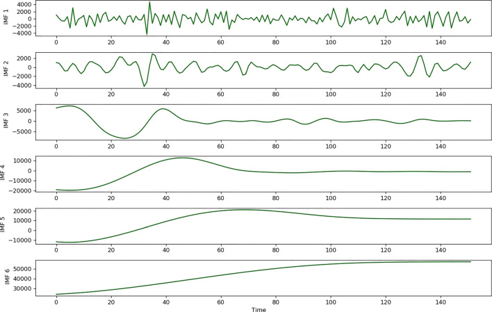
In this paper, we collected the number of confirmed cases in Wuhan from January 1 to May 29, a total of 150 days of data. We use EEMD to decompose the time series data into six IMF components. The epidemic data and IMF components are shown in Fig. 8.

Fig. 8.

The Decomposition Results of EEMD

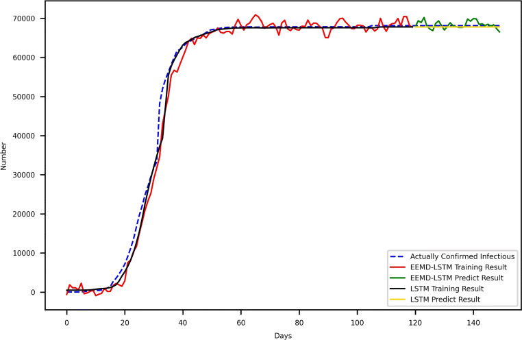
We select the data of the first 120 days of each IMF component as the training set and input them into an LSTM respectively, and the weighted sum of the output results of the final six LSTM models is used as the final output result. In this paper, the LSTM model uses the Keras framework and sets the time step to 2 (that is, the data of the first two days are used to predict the data of the third day). The Adam optimizer is selected, the loss function is the MSE, which is $Loss=\frac{1}{n}{\sum }_{i=1}^n{(y_{prediction}^{\left(i\right)}-y_{true}^{\left(i\right)})}^2$, the iteration is 200 times and the batch size is 1. Then, we use the trained model to predict the data for the next 30 days and compared it with the LSTM model and actual data, as shown in Fig. 9. However, we have found that EEMD-LSTM has a certain effect in short-term predictive ability, but it can’t obtain useful information on long-term trends like SEIR and other models based on infectious disease theory. For example, if the current epidemic data does not show a significant downward trend, then the prediction based on LSTM will basically maintain a growing trend. Moreover, the independent and identical distribution of data is emphasized in the deep learning model. For example, even if the audio signal is different from different people, it is generally consistent with a high degree of distribution and can be summarized. However, due to the greater influence of policy and other factors, the epidemic data does not have sufficient consistency. From this point of view, in the model based on the theory of infectious diseases, we can estimate the model parameters based on the previous data and reasonable assumptions, so as to make a more reasonable deduction of the epidemic trend.

Fig. 9.

The Prediction Result of EEMD-LSTM for Confirmed Patients

Conclusion

Based on epidemiological knowledge, the transmission characteristics and the actual occurrences of isolated observations of confirmed patients and susceptible patients, this paper establishes a COVID-19 epidemic control model based on isolation measures, analyses the effect of isolated centralized diagnosis and treatment, and makes a certain prediction of epidemic development. By comparing with actual data, our model can effectively predict the peak and scale of the COVID-19 epidemic to a certain extent. With the increase in the intensity of prevention and control measures, the peak number of confirmed cases will gradually decrease, and it will help to reach the peak point earlier.

Bo Huang

was born in Hubei, China, in 1985. He received M.Sc. degree (2010) and Ph.D. degree (2014) in Computer Science from Wuhan University, Wuhan, Hubei, China. He is currently an Associate Professor at Shanghai University of Engineering Science(SUES). His current research interests include artificial intelligence, machine learning, data analytics, and the application of soft computing.

References

- 1.Lee JS, Park S, Jeong HW, et al. (2020) Immunophenotyping of COVID-19 and influenza highlights the role of type I interferons in development of severe COVID-19. Sci Immunology 5(49) [DOI] [PMC free article] [PubMed]
- 2.Cai YL, Kang Y, Wang WM. A stochastic SIRS epidemic model with nonlinear incidence rate. Appl Math Comput. 2017;305:221–240. [Google Scholar]
- 3.Almeida R. Analysis of a fractional SEIR model with treatmen. Appl Math Lett. 2018;84:56–62. doi: 10.1016/j.aml.2018.04.015. [DOI] [Google Scholar]
- 4.He SB, Peng YX, Sun KH. SEIR Modeling of the COVID-19 and its dynamics. Nonlinear Dynam. 2020;101(3):1667–1680. doi: 10.1007/s11071-020-05743-y. [DOI] [PMC free article] [PubMed] [Google Scholar]
- 5.Iwata K, Miyakoshi C. A simulation on potential secondary spread of novel coronavirus in an exported country using a stochastic epidemic SEIR model. J Clinic Med. 2020;9(4):944. doi: 10.3390/jcm9040944. [DOI] [PMC free article] [PubMed] [Google Scholar]
- 6.Wu JT, Leung K, Leung GM. Nowcasting and forecasting the potential domestic and international spread of the 2019-nCoV outbreak originating in Wuhan, china: A modelling study. Lancet. 2020;395(10225):689–697. doi: 10.1016/S0140-6736(20)30260-9. [DOI] [PMC free article] [PubMed] [Google Scholar]
- 7.Wang X, Tang SY, Chen Y, Feng XM, Xiao YN, Xu ZB. When will be the resumption of work in Wuhan and its surrounding areas during COVID-19 epidemic? A data-driven network modeling analysis. Scientia Sinica Math. 2020;50(7):969–978. doi: 10.1360/SSM-2020-0037. [DOI] [Google Scholar]
- 8.Hernandez-Matamoros A, Fujita H, Hayashi T, Perez-Meana H. Forecasting of COVID-19 per regions using ARIMA models and polynomial functions. Appl Soft Comput. 2020;96:106610. doi: 10.1016/j.asoc.2020.106610. [DOI] [PMC free article] [PubMed] [Google Scholar]
- 9.Catelli R, Gargiulo F, Casola V, De Pietro G, Fujita H, Esposito M. Crosslingual named entity recognition for clinical de-identification applied to a COVID-19 Italian data set. Appl Soft Comput. 2020;97:106779. doi: 10.1016/j.asoc.2020.106779. [DOI] [PMC free article] [PubMed] [Google Scholar]
- 10.Fu H, Wang HW, Xi XY, et al. And Database of epidemic trends and control measures during the first wave of COVID-19 in mainland China. Int J Infect Dis. 2021;102:463–471. doi: 10.1016/j.ijid.2020.10.075. [DOI] [PMC free article] [PubMed] [Google Scholar]
- 11.Abbasi Z, Zamani I, Mehra AHA, Shafieirad M. Ibeas A. Optimal control design of impulsive SQEIAR epidemic models with application to COVID-19. Chaos Solitons Fractals. 2020;139:110054. doi: 10.1016/j.chaos.2020.110054. [DOI] [PMC free article] [PubMed] [Google Scholar]
- 12.Prem K, Liu Y, Russell TW, Kucharski AJ, et al. And The effect of control strategies to reduce social mixing on outcomes of the COVID-19 epidemic in Wuhan, china: A modelling study. Lancet Public Health. 2020;5(5):e261–e270. doi: 10.1016/S2468-2667(20)30073-6. [DOI] [PMC free article] [PubMed] [Google Scholar]
- 13.Zhu CC, Zhu J. Dynamic analysis of a delayed COVID-19 epidemic with home quarantine in temporal-spatial heterogeneous via global exponential attractor method. Chaos Solitons Fractals. 2021;143:110546. doi: 10.1016/j.chaos.2020.110546. [DOI] [PMC free article] [PubMed] [Google Scholar]
- 14.Yan C, Wu LF, Liu LY, Zhang K. Fractional Hausdorff grey model and its properties. Chaos Solitons Fractals. 2020;109915:138. [Google Scholar]
- 15.Rothan HA, Byrareddy SN. The epidemiology and pathogenesis of coronavirus disease (COVID-19) outbreak. J Autoimmun. 2020;102433:109. doi: 10.1016/j.jaut.2020.102433. [DOI] [PMC free article] [PubMed] [Google Scholar]
- 16.Liu Z. Dynamics of positive solutions to SIR and SEIR epidemic models with saturated incidence rates. Nonlinear Anal Real World Appl. 2013;14(3):1286–1299. doi: 10.1016/j.nonrwa.2012.09.016. [DOI] [Google Scholar]
- 17.Wu Q, Xiao G. A colored mean-field model for analyzing the effects of awareness on epidemic spreading in multiplex networks. Chaos An Interdiscip J Nonlinear Sci. 2018;28(10):103116. doi: 10.1063/1.5046714. [DOI] [PubMed] [Google Scholar]
- 18.Cao WJ, Liu XF, Han Z, et al. Statistical analysis and autoregressive modeling of confirmed coronavirus disease 2019 epidemic cases. Acta Physica Sinica. 2020;69(9):090203. doi: 10.7498/aps.69.20200503. [DOI] [Google Scholar]
- 19.Machida M, Nakamura I, Saito R, et al. And Adoption of personal protective measures by ordinary citizens during the COVID-19 outbreak in Japan. Int J Infect Dis. 2020;94:139–144. doi: 10.1016/j.ijid.2020.04.014. [DOI] [PMC free article] [PubMed] [Google Scholar]
- 20.Wilder-Smith A, Freedman DO. Isolation, quarantine, social distancing and community containment: Pivotal role for old-style public health measures in the novel coronavirus (2019-nCoV) outbreak. J Travel Med. 2020;27(2):taaa020. doi: 10.1093/jtm/taaa020. [DOI] [PMC free article] [PubMed] [Google Scholar]
- 21.Alfaro-Murillo JA, Feng Z, Glasser JW. Analysis of an epidemiological model structured by time-since-last-infection. J Different Equ. 2019;267(10):5631–5661. doi: 10.1016/j.jde.2019.06.002. [DOI] [PMC free article] [PubMed] [Google Scholar]
- 22.Bashkirtseva I, Ryashko L, Ryazanova T. Analysis of regular and chaotic dynamics in a stochastic eco-epidemiological model. Chaos Solitons Fractals. 2020;131:109549. doi: 10.1016/j.chaos.2019.109549. [DOI] [Google Scholar]
- 23.Britton T, Ouédraogo D. SEIRS Epidemics with disease fatalities in growing populations. Math Biosci. 2018;296:45–59. doi: 10.1016/j.mbs.2017.11.006. [DOI] [PubMed] [Google Scholar]
- 24.Liu Y, Gayle AA, Wilder-Smith A, et al. And The reproductive number of COVID-19 is higher compared to SARS coronavirus. J Travel Med. 2020;27(2):taaa021. doi: 10.1093/jtm/taaa021. [DOI] [PMC free article] [PubMed] [Google Scholar]
- 25.Annas S, Pratama MI, Rifandi M, et al. And Stability analysis and numerical simulation of SEIR model for pandemic COVID-19 spread in indonesia. Chaos Solitons Fractals. 2020;110072:139. doi: 10.1016/j.chaos.2020.110072. [DOI] [PMC free article] [PubMed] [Google Scholar]
- 26.Zhang XY, Ruan ZY, Zheng MH, Barzel B, Boccaletti S. Epidemic spreading under infection-reduced-recovery. Chaos Solitons Fractals. 2020;140:110130. doi: 10.1016/j.chaos.2020.110130. [DOI] [Google Scholar]
- 27.Jin T, Li Q, Mohamed MA. A novel adaptive EEMD method for switchgear partial discharge signal denoising. IEEE Access. 2019;7:58139–58147. doi: 10.1109/ACCESS.2019.2914064. [DOI] [Google Scholar]
- 28.Li R, Pei S, Chen B, et al. And Substantial undocumented infection facilitates the rapid dissemination of novel coronavirus (SARS-CoV-2) Science. 2020;368(6490):489–493. doi: 10.1126/science.abb3221. [DOI] [PMC free article] [PubMed] [Google Scholar]
- 29.Lai CC, Shih TP, Ko WC, et al. Severe acute respiratory syndrome coronavirus 2 (SARS-CoV-2) and coronavirus disease-2019 (COVID-19): The epidemic and the challenges. Int J Antimicrob Agents. 2020;55(3):105924. doi: 10.1016/j.ijantimicag.2020.105924. [DOI] [PMC free article] [PubMed] [Google Scholar]
- 30.Mohamadou Y, Halidou A, Kapen PT. A review of mathematical modeling, artificial intelligence and datasets used in the study, prediction and management of COVID-19. Appl Intell. 2020;50(11):3913–3925. doi: 10.1007/s10489-020-01770-9. [DOI] [PMC free article] [PubMed] [Google Scholar]
- 31.Tang B, Wang X, Li Q, et al. And Estimation of the transmission risk of the 2019-nCoV and its implication for public health interventions. J Clinic Med. 2020;9(2):462. doi: 10.3390/jcm9020462. [DOI] [PMC free article] [PubMed] [Google Scholar]