Fig. 6. A systematic comparison of R loop CUT&Tag versus other conventional R loop mapping methods.

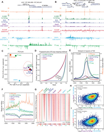
(A and B) Track examples of HEK293T PRO-seq, GST-His₆-2×HBD CUT&Tag, S9.6 CUT&Tag, MapR (26), R-ChIP (24), DRIPc-seq (34), and TT-seq signals at the HSPD1 (A) and GRK6 (B) loci. The reads were aligned to the human hg38 genome, and the signals were normalized by reads per million. (C) PCA plot showing R loop CUT&Tag, MapR, and R-ChIP clustered together. (D) Fingerprint plots of R loop CUT&Tag, MapR, and R-ChIP. w.r.t., with respect to. (E and F) Metaplots of signals detected by different R loop mapping methods, PRO-seq, and TT-seq around the 2-kb window of the TSSs and TESs. Strand-specific signals from PRO-seq, TT-seq, DRIPc-seq, and R-ChIP were used for plotting. (G) Heatmap analysis of PRO-seq, TT-seq, and R loop mapping methods at the TSS of transcriptionally active genes (the reads per million of PRO-seq signals at TSS, >1; n = 13,220). The heatmaps are sorted by the GST-His₆-2×HBD CUT&Tag signals. R loop CUT&Tag assays, MapR, and R-ChIP have enrichment at the TSS, while DRIPc-seq does not show this trend. (H and I) Scatter plots of R loop CUT&Tag and MapR reads per kilobase, per million mapped reads (RPKM) values (H) or R-ChIP RPKM values (I) at TSS. The r values were calculated by Pearson correlation.